Data Structures and Sequences

Lecture W1W1: Interfaces, Arrays, Linked Lists, and Amortization

Lucas P. Cordova, Ph.D.

Willamette University

August 26, 2026

Before we begin: HW0

The short version of Tuesday’s announcement

HW0 samples the kinds of math this course draws on. Your previous courses covered these topics to different depths and with different notation; I am not assuming you have seen every piece of it before.
It is a diagnostic, not a gatekeeper: it shows you what to dust off, and it shows me how to pace the course to the room.
It does not count toward your final grade. You will get it back scored out of 100, but that number is feedback for you and calibration for me.
It is also your practice run with LaTeX and the Canvas submission workflow before the graded homework begins.
Looking up notation or a definition is expected and fine; work the problems themselves on your own.

Stuck after a refresher? Come to Student Hours (MW 10:15 - 11:15 AM, T/Th 11:15 AM - 12:15 PM) or Sam’s help hours (Sun 3:00 - 6:00 PM, Fri 3:00 - 4:30 PM at the QUAD).

A quick tour of what HW0 asks

Six problems, six kinds of background. Let’s put the notation for each back on the table.

Problem	Background it exercises
1	Set notation and operations
2	Probability and expected value
3	Modular arithmetic
4	Proof by induction
5	Graph vocabulary + induction
6	Python and the word “subarray”

Refresher: sets

Set-builder notation: \(\{ 2i \mid i \in \mathbb{Z} \text{ and } 1 \leq i \leq 3 \} = \{2, 4, 6\}\): “the set of values \(2i\), as \(i\) ranges over the integers 1 to 3.”
Operations: \(A \cap B\) (in both), \(A \cup B\) (in either), \(A - B\) (in \(A\) but not \(B\)); \(\lvert A \rvert\) is the number of elements.
The binomial coefficient \(\binom{n}{k}\), read “\(n\) choose \(k\)”: the number of ways to choose \(k\) items from \(n\), \(\binom{n}{k} = \frac{n!}{k!\,(n-k)!}\). Example: \(\binom{4}{2} = 6\).

Refresher: expectation and mod

A random variable \(X\) takes values with probabilities; the expected value \(\mathrm{E}[X]\) is the average of those values weighted by probability: \(\mathrm{E}[X] = \sum_x x \cdot \Pr[X = x]\).
One fair six-sided die: \(\mathrm{E}[X] = \frac{1+2+3+4+5+6}{6} = 3.5\).
Linearity of expectation: \(\mathrm{E}[X + Y] = \mathrm{E}[X] + \mathrm{E}[Y]\), always, with no independence required. It is the single most useful fact on the problem.
Mod: \(a \bmod m\) is the remainder when \(a\) is divided by \(m\) (\(17 \bmod 5 = 2\)). And \(a \equiv b \pmod{m}\) means \(m\) divides \(a - b\): check the difference, not the numbers.

Refresher: induction and graphs

An induction proof has exactly two jobs: a base case (verify the smallest instance directly) and an inductive step (assume it holds for \(n\), show it holds for \(n+1\)). State both, every time.
A graph \(G = (V, E)\) is vertices plus edges; the degree of a vertex is how many edges touch it.
A path walks along edges; a cycle is a path that returns to its start; acyclic means no cycles; connected means every vertex can reach every other.
For Problem 6: a subarray is a consecutive run of array elements. \((2, 7)\) is a subarray of \((5, 2, 7, 1)\); \((5, 7)\) is not (that is a subsequence).

You’re saying words, but…

If any of these felt brand new rather than rusty, tell me on HW0 by doing your honest best, and come see me or Sam this week.

Learning objectives

What you will leave with

By the end of this session, you will be able to:

Distinguish an interface (what operations are promised) from a data structure (how they are delivered), and explain why the separation matters.
State the Sequence interface and recognize stacks and queues as special cases of it.
Derive the worst-case cost of each sequence operation for static arrays and linked lists from the word-RAM model.
Explain how dynamic arrays achieve amortized \(O(1)\) appends, and what “amortized” does and does not promise.
Choose the right sequence implementation for a workload, and defend the choice with the cost table.

Where we left off

On Monday we agreed on the rules of the game:

An algorithm solves a problem if it returns a correct output for every input, and we prove that with induction.
We measure efficiency by counting operations as a function of input size \(n\), not by timing programs.
In the word-RAM model, arithmetic, comparisons, and reading or writing one machine word of memory each cost \(O(1)\).

Today we use those rules to answer a new question: how should a program remember things?

Interfaces vs. data structures

Two different questions

Interface. A specification: which operations on stored data are supported, and what each one returns. Also called an API or an abstract data type.

Data structure. A representation: how the data is laid out in memory, with an algorithm for each supported operation.

The interface states the problem; the data structure is a solution.
One interface can have many data structures behind it, with very different costs.
This mirrors Monday’s lesson: problems and algorithms are different things, and so are interfaces and implementations.

The two interfaces of this course

Nearly everything we build this semester supports one of two contracts:

Interface	Order is…	Signature question
Sequence	extrinsic: you put items at positions	“what is the \(i\)th item?”
Set	intrinsic: items carry keys	“do you hold an item with key \(k\)?”

Today: Sequence. Next week: Set, via hashing.

The Sequence interface

The contract

Maintain an ordered collection \((x_0, x_1, \ldots, x_{n-1})\) of \(n\) items, with:

Group	Operation	Meaning
Container	`build(X)`	build a sequence from the items in iterable `X`
	`len()`	return \(n\)
Static	`get_at(i)`, `set_at(i, x)`	read or replace the \(i\)th item
Dynamic	`insert_at(i, x)`, `delete_at(i)`	add or remove at position \(i\)
	`insert_first(x)`, `delete_first()`	add or remove at the front
	`insert_last(x)`, `delete_last()`	add or remove at the back

The interface says nothing about memory. That is the data structure’s job.

You already know two special cases

A stack and a queue are just sequences that promise fewer operations:

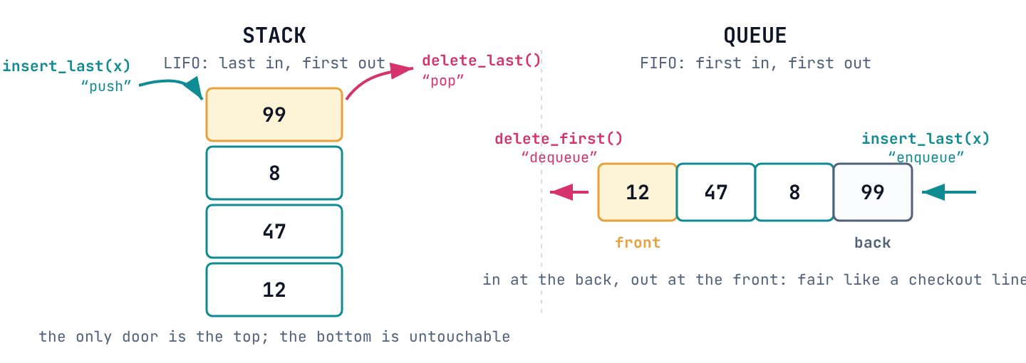
Restricting an interface is powerful: the fewer operations you promise, the faster the implementation you can pick.

When a problem does not need an operation, do not pay for it.

Implementation 1: the static array

Arrays are the memory model made visible

An array of \(n\) items is \(n\) consecutive machine words, so finding item \(i\) is arithmetic, not searching:

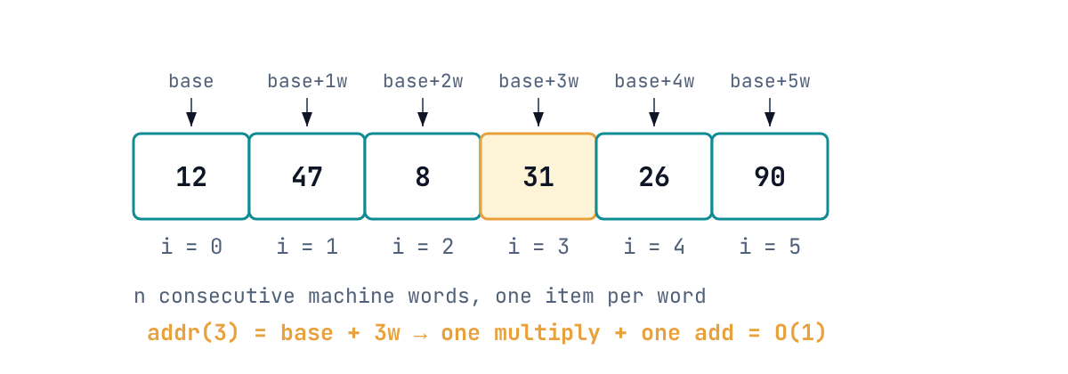
get_at(i) and set_at(i, x) run in \(\Theta(1)\) worst-case time. This is the array’s superpower.

…but order is rigid

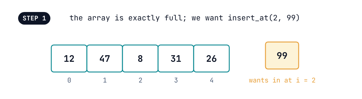
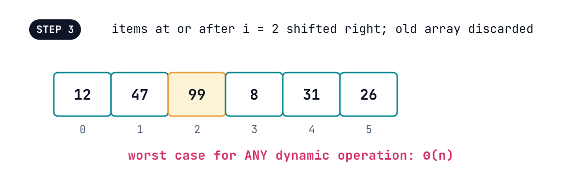
So every dynamic operation costs \(\Theta(n)\) in the worst case, even at the back, and even at the front.

Implementation 2: the linked list

Trade addresses for pointers

A linked list stores each item in a node with two fields: node.item and node.next. The structure keeps one pointer, head, to the first node.

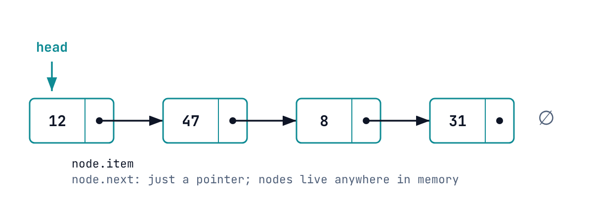
The price of this freedom: to reach item \(i\) you must walk the chain, so get_at(i) costs \(O(n)\).

A linked list is not a Python list. Python’s list is a dynamic array, which is coming up.

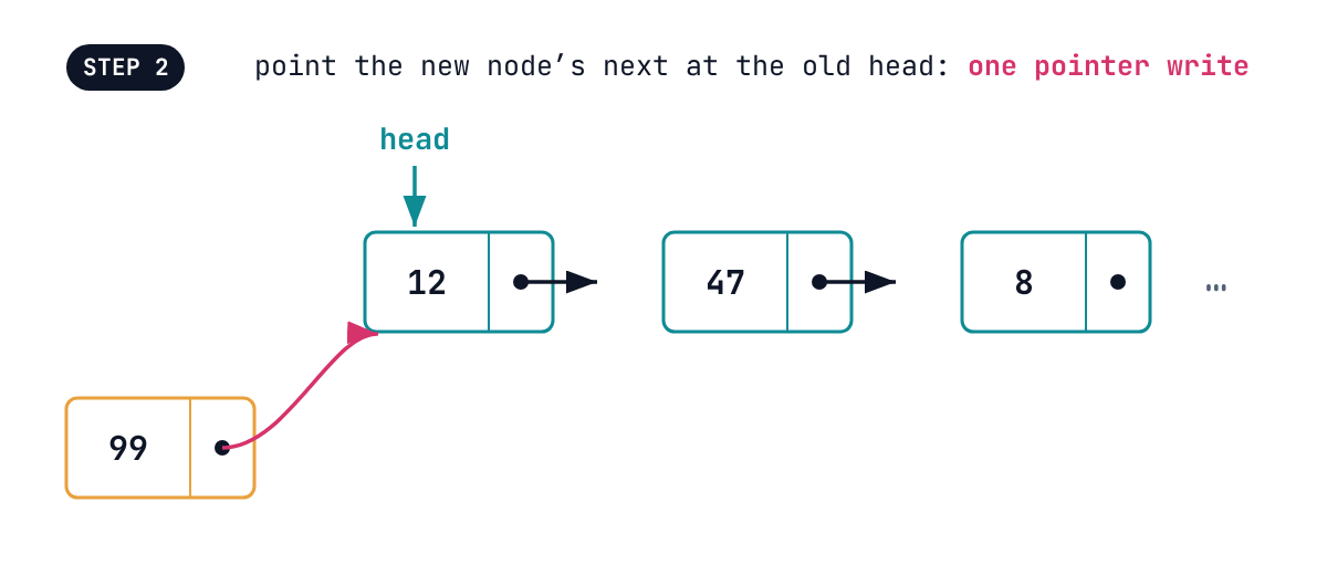
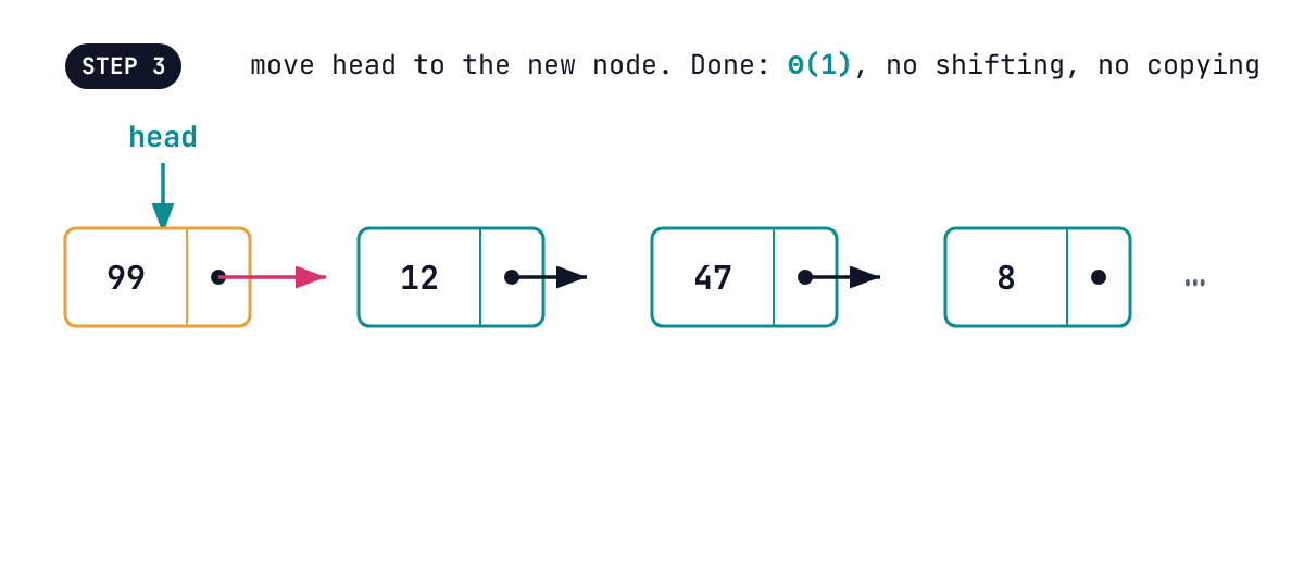
`insert_first`, one frame at a time

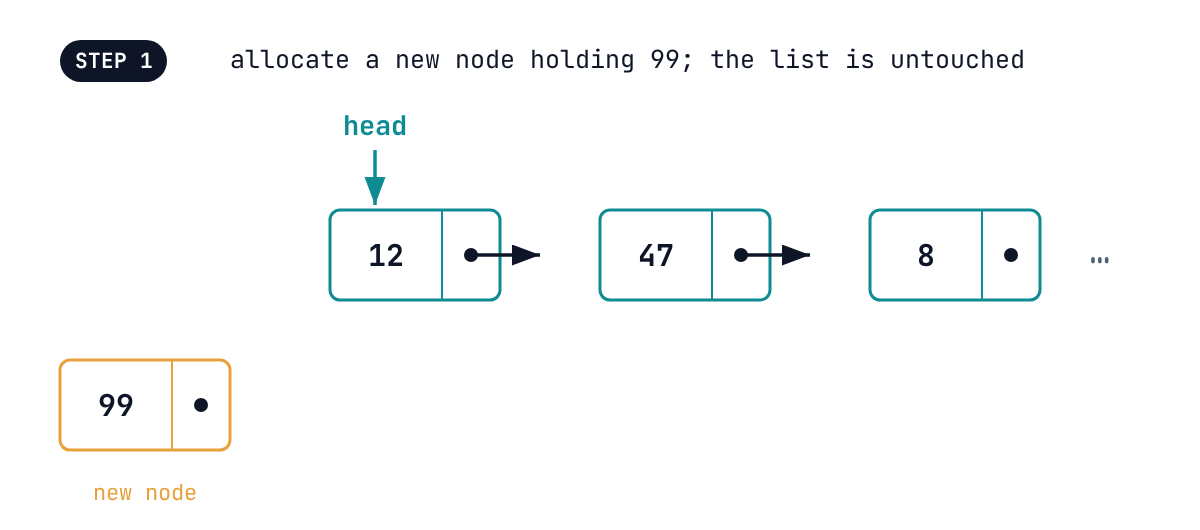
Two pointer writes, no shifting, no reallocation, and \(n\) never mattered: \(\Theta(1)\) worst case.

Activity: fill in the scorecard

With your neighbor, fill in the worst-case cost, \(O(1)\) or \(O(n)\), of each cell:

Operation	Array	Linked list
`get_at(i)` / `set_at(i, x)`
`insert_first(x)` / `delete_first()`
`insert_last(x)` / `delete_last()`
`insert_at(i, x)` / `delete_at(i)`

Then answer: which workload makes the array win, and which makes the list win?

3 minutes.

The scorecard so far

Operation, worst case	Array	Linked list
`build(X)`	\(O(n)\)	\(O(n)\)
`get_at(i)`, `set_at(i, x)`	\(O(1)\)	\(O(n)\)
`insert_first(x)`, `delete_first()`	\(O(n)\)	\(O(1)\)
`insert_last(x)`, `delete_last()`	\(O(n)\)	\(O(n)\)
`insert_at(i, x)`, `delete_at(i)`	\(O(n)\)	\(O(n)\)

Each structure is excellent at exactly one thing. Can we get the best of both worlds?

Implementation 3: the dynamic array

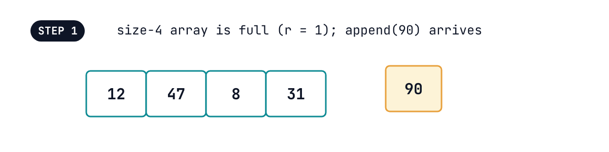
The idea: over-allocate

Drop the “exactly full” invariant: allocate extra space so most appends need no reallocation.
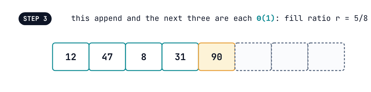
Define the fill ratio \(r = n / (\text{allocated size})\), with \(0 \leq r \leq 1\).
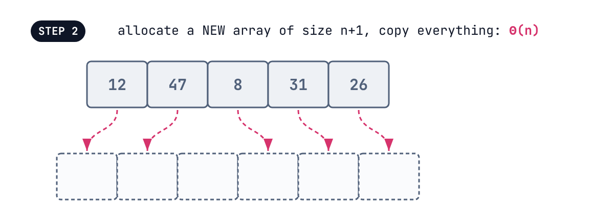
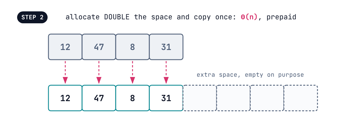
When the array fills (\(r = 1\)), reallocate to a bigger array, say twice the size, and copy everything over: one expensive \(\Theta(n)\) operation.
After that resize, the next \(\Theta(n)\) appends are each \(\Theta(1)\): the expensive copy has been prepaid.

Doubling, one frame at a time

Counting the total cost of \(n\) appends

Start empty and append \(n\) times with doubling. Resizes happen at sizes \(1, 2, 4, 8, \ldots\), so the total copying work is

\[1 + 2 + 4 + \cdots + 2^{\lfloor \log_2 n \rfloor} \;<\; 2n \;=\; \Theta(n).\]

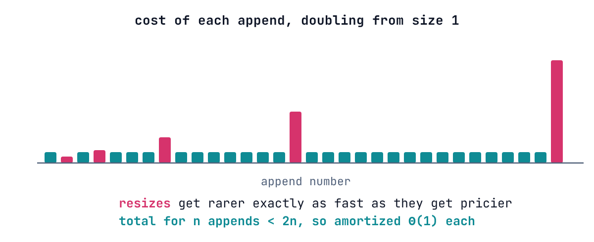
Any sequence of \(n\) appends costs \(\Theta(n)\) total, even though single appends occasionally cost \(\Theta(n)\). The geometric series does the work: each resize doubles the distance to the next one.

Amortized analysis

An operation has amortized cost \(T(n)\) if any sequence of \(k\) operations costs at most \(k \cdot T(n)\) in total.

Appending to a dynamic array is amortized \(\Theta(1)\): \(\Theta(1)\) “on average” over any run of operations.
Amortized is a guarantee about totals, not about individual operations; one append can still pause to copy everything.
This is our third notion of cost this week: worst case, amortized, and, when we reach hashing, expected.

Deleting without wasting space

delete_last() alone is \(\Theta(1)\): decrement \(n\). But after many deletes the array is mostly empty, and we promised \(\Theta(n)\) space.
Tempting fix: shrink as soon as the array is exactly full. Then alternating insert and delete resizes every time: \(\Theta(n)\) per operation. Bad.
Right fix: shrink only when the fill ratio drops below \(r_d\) (say \(1/4\)), and resize to a comfortable ratio \(r_i\) (say \(1/2\)).
With a gap between \(r_d\) and \(r_i\), there must be \(\Theta(n)\) cheap operations between expensive resizes, so the amortized cost stays \(\Theta(1)\).

This is your Python list

Python’s list is a dynamic array: append and pop are amortized \(O(1)\).
insert(0, x), pop(0), and del L[i] shift items: \(O(n)\). A loop that does pop(0) \(n\) times is \(\Theta(n^2)\).
When you need fast operations at the front, reach for a different structure, not a bigger machine.

from collections import deque   # doubly-ended queue

line = deque()
line.append("task A")           # O(1) at the back
line.appendleft("urgent task")  # O(1) at the front
line.popleft()                  # O(1) at the front

The final scorecard

Operation, worst case	Array	Linked list	Dynamic array
`build(X)`	\(O(n)\)	\(O(n)\)	\(O(n)\)
`get_at(i)`, `set_at(i, x)`	\(O(1)\)	\(O(n)\)	\(O(1)\)
`insert_first(x)`, `delete_first()`	\(O(n)\)	\(O(1)\)	\(O(n)\)
`insert_last(x)`, `delete_last()`	\(O(n)\)	\(O(n)\)	\(O(1)\) amortized
`insert_at(i, x)`, `delete_at(i)`	\(O(n)\)	\(O(n)\)	\(O(n)\)

There is no free lunch, only informed trade-offs. Naming the workload first tells you which column to buy.

A look ahead: the Set interface

When order comes from the data

A Set maintains items with unique keys (item x has key x.key) and supports:

Group	Operation	Meaning
Container	`build(X)`, `len()`	as before
Static	`find(k)`	return the item with key \(k\)
Dynamic	`insert(x)`, `delete(k)`	add or remove by key
Order	`find_min()`, `find_max()`, `find_next(k)`, `find_prev(k)`	navigate by key order

A dictionary is a Set without the Order operations; Python’s dict is one.
With today’s structures, find(k) seems doomed to \(O(n)\): check every item.
After the long weekend we will do much, much better, and the answer is one of the great ideas of computer science: hashing.

Wrap-up

The one-slide version

Interfaces are problems; data structures are solutions. Arrays buy \(O(1)\) random access with rigid order, linked lists buy \(O(1)\) front edits with slow access, and dynamic arrays buy amortized \(O(1)\) appends by prepaying resizes. Choose by workload, and read the fine print on “amortized.”

What’s next

Next week at a glance

Topics: Sorting (insertion sort, merge sort) and divide and conquer: recurrences and the Master Theorem. The sequence operations you priced today become the inner loops.

Supplemental reading (highly recommended): CLRS Chapter 2, in your own copy or online through Canvas/Perusall.

Upcoming deliverables:

HW0 due Monday, August 31 at 9:59 PM, via Canvas (PDF + your Python file).
HW1 assigned Monday.

References

Sources

Cormen, T. H., Leiserson, C. E., Rivest, R. L., and Stein, C. Introduction to Algorithms, 4th edition, MIT Press. Chapters 10 and 16.4.
CS 351 Syllabus: Canvas.
Python Software Foundation. Time Complexity, wiki.python.org/moin/TimeComplexity.