Sorting
Lecture W2M1: Insertion Sort, Merge Sort, and What They Cost
August 31, 2026
Learning objectives
What you will leave with
By the end of this class, you will be able to:
- State the sorting problem precisely, and explain why brute force is correct but hopeless.
- Prove insertion sort correct with an invariant and induction, and derive its \(\Theta(n^2)\) worst-case cost.
- Explain merge sort as divide and conquer, and why the two-finger merge costs \(O(n)\).
- Build the recursion tree for \(T(n) = 2T(n/2) + c \cdot n\) and read \(\Theta(n \log n)\) off of it.
- Choose between insertion sort and merge sort for a given workload, and defend the choice.
Last Wednesday
We concluded by mentioning the Set interface, which stores items by key and its questions are about values, not positions: find(k), find_min(), find_max(), find_next(k). 🛍️
- Store the items in an array in arbitrary order and try
find_min(): you must examine all \(n\) cells, because any cell you skip could be hiding the minimum. That is \(\Theta(n)\), and no cleverness avoids it. find(k)has the same problem: a position tells you nothing about which key lives there, so the search scans until it finds \(k\) or runs out. \(O(n)\) again.- The array is not the culprit; the arbitrary order is. When positions carry no information about values, every value question forces a full scan.
Order is information
If the very same items sat in an array sorted by key, positions would suddenly mean something, and every Set question gets cheaper:
| Operation | Unsorted array | Sorted array |
|---|---|---|
find_min(), find_max() |
\(O(n)\) | \(O(1)\): look at the ends |
find(k) |
\(O(n)\) | \(O(\log n)\): binary search |
find_next(k), find_prev(k) |
\(O(n)\) | \(O(\log n)\) |
find_min() is the cleanest example: sorted order pins the minimum to index \(0\), so the scan that was unavoidable becomes a single read.
The missing piece is the one this table quietly assumes: someone has to put the array in sorted order first. Today we ask how, and at what cost.
The sorting problem
The problem, stated precisely
Sorting. Given an array \(A\) of \(n\) numbers, output an array \(B\) that is a permutation of \(A\) (same elements, possibly reordered) and is sorted: \(B[i-1] \leq B[i]\) for every \(i \in \{1, \ldots, n-1\}\).
- Example: \((7, 3, 9, 2, 6) \rightarrow (2, 3, 6, 7, 9)\).
- Both halves of the contract matter: \((1, 2, 3)\) is sorted but is not a permutation of \((7, 3, 9)\), and returning \(A\) unchanged is a permutation but is not sorted.
- Two useful labels: a sort is destructive if it overwrites \(A\), and in place if it uses only \(O(1)\) extra space beyond the array.
Problem, not algorithm
Sorting is a problem, not an algorithm. Monday of week 1 taught us to keep those separate, and today we dance with three different algorithms for this one problem. 💃🏼
First idea: try every ordering
The specification practically dares us: some permutation of \(A\) is sorted, so check them all.
- Correct? Yes, by brute force: a sorted permutation exists, and we will not stop until we find one.
- Fast? There are \(n!\) permutations, and checking one costs \(\Theta(n)\), so the worst case is \(\Omega(n! \cdot n)\).
- At \(n = 20\) that is more than \(10^{19}\) checks. At one billion per second: several centuries. 🤯
Cost matters
Correctness is not enough. This course exists because of the gap between an answer and an answer you can afford.
Insertion sort
The card player’s algorithm
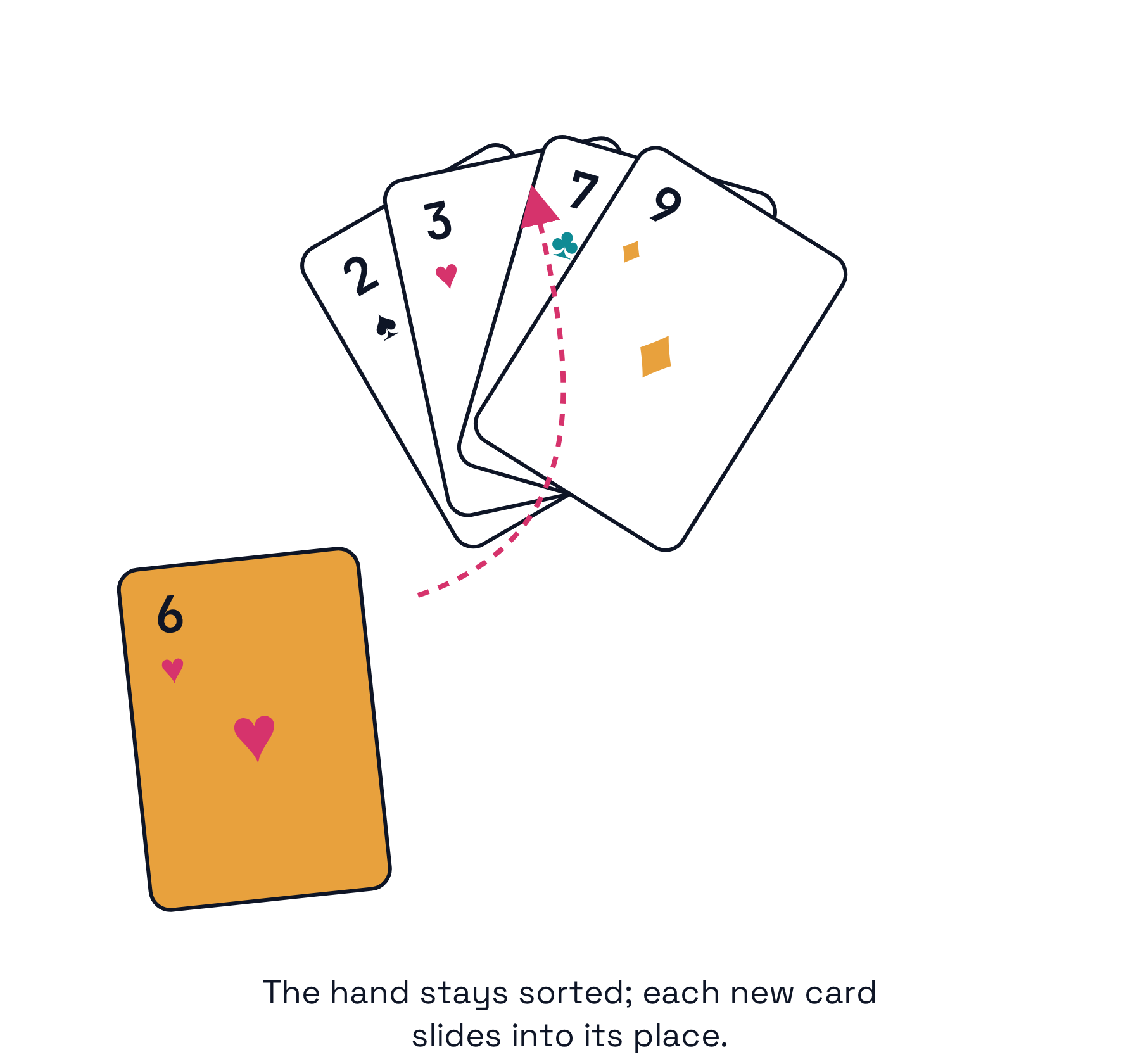
You already run this algorithm when you pick up a hand of cards: keep the cards you hold sorted, and tuck each new card into its place.
| Round | Array | What happened |
|---|---|---|
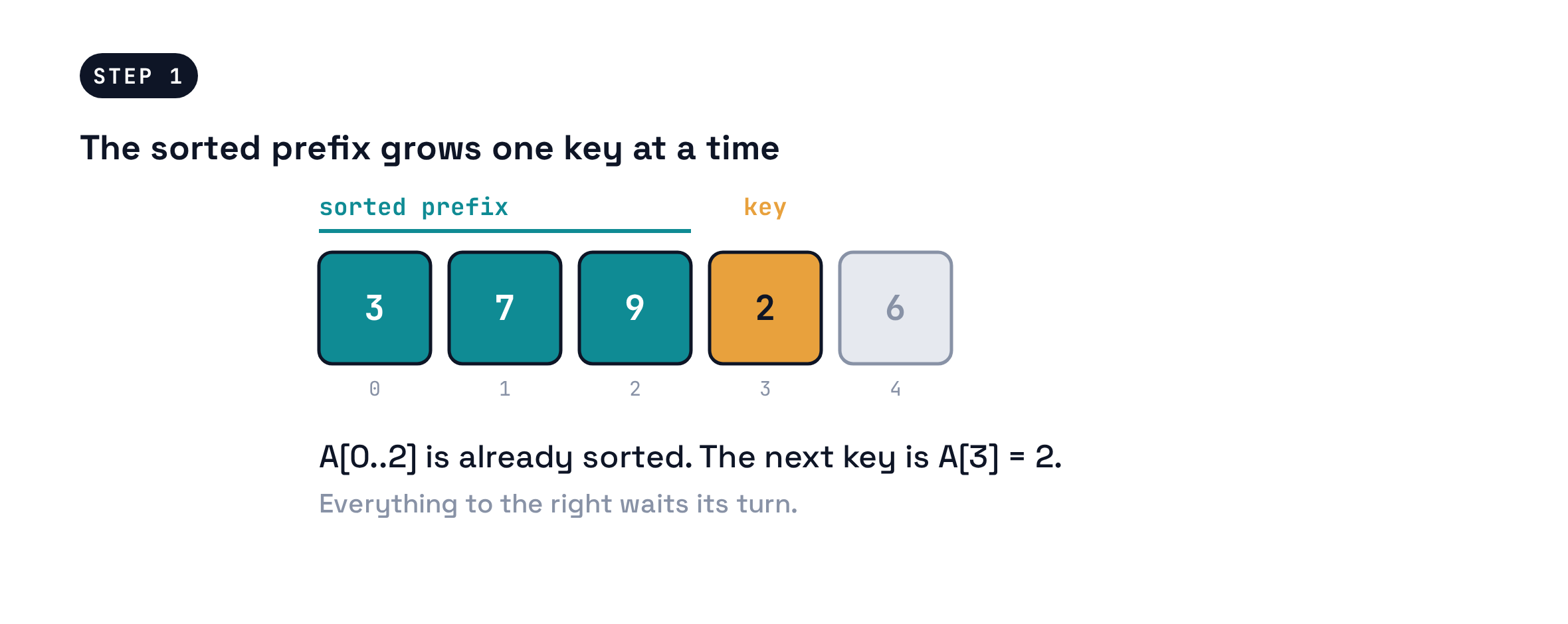
| start | \((7, 3, 9, 2, 6)\) | \(A[0]\) alone is sorted |
| \(i = 1\) | \((3, 7, 9, 2, 6)\) | key \(3\) moved left past \(7\) |
| \(i = 2\) | \((3, 7, 9, 2, 6)\) | key \(9\) already in place |
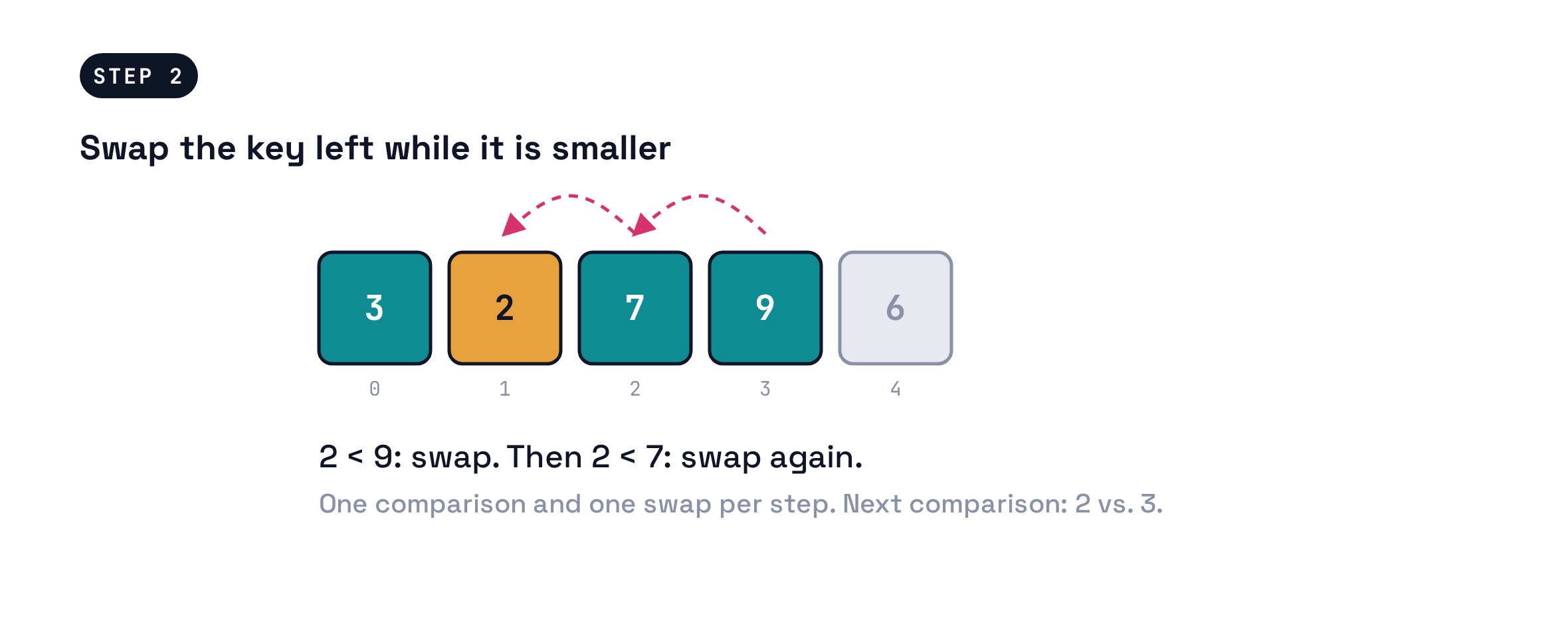
| \(i = 3\) | \((2, 3, 7, 9, 6)\) | key \(2\) moved left past \(9, 7, 3\) |
| \(i = 4\) | \((2, 3, 6, 7, 9)\) | key \(6\) moved left past \(9, 7\) |
One sentence: grow a sorted prefix, one key at a time.
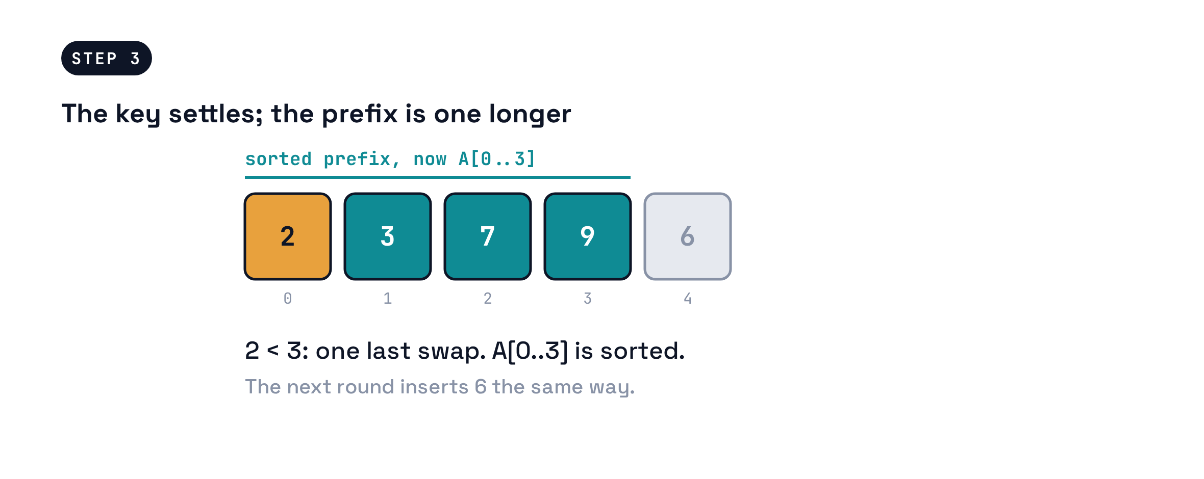
One insertion, frame by frame
The code
- Destructive and in place: the only extra storage is the counters.
- Round \(i\) does at most \(i\) comparisons and \(i\) swaps, each \(O(1)\) in the word-RAM model.
- No round undoes earlier work, which is the claim we now have to actually prove.
Correctness is an induction
Invariant. At the start of the round that inserts key \(A[i]\), the prefix \(A[0..i-1]\) is sorted.
- Base case (\(i = 1\)): the prefix \(A[0]\) has one element, so it is sorted.
- Inductive step: assume \(A[0..i-1]\) is sorted. The inner loop swaps the key left exactly until the neighbor to its left is no larger. Every element that was to the left stays in order, so afterward \(A[0..i]\) is sorted.
- Conclusion: when the loop ends at \(i = n\), the invariant says \(A[0..n-1]\), the whole array, is sorted. And the array is always a permutation of the input, because swaps never create or destroy elements.
Key to all correctness proofs
Every correctness proof this semester will have this base-case-plus-inductive-step shape.
The bill for insertion sort
Worst case, the key travels all the way left every round (a reverse-sorted input does exactly this):
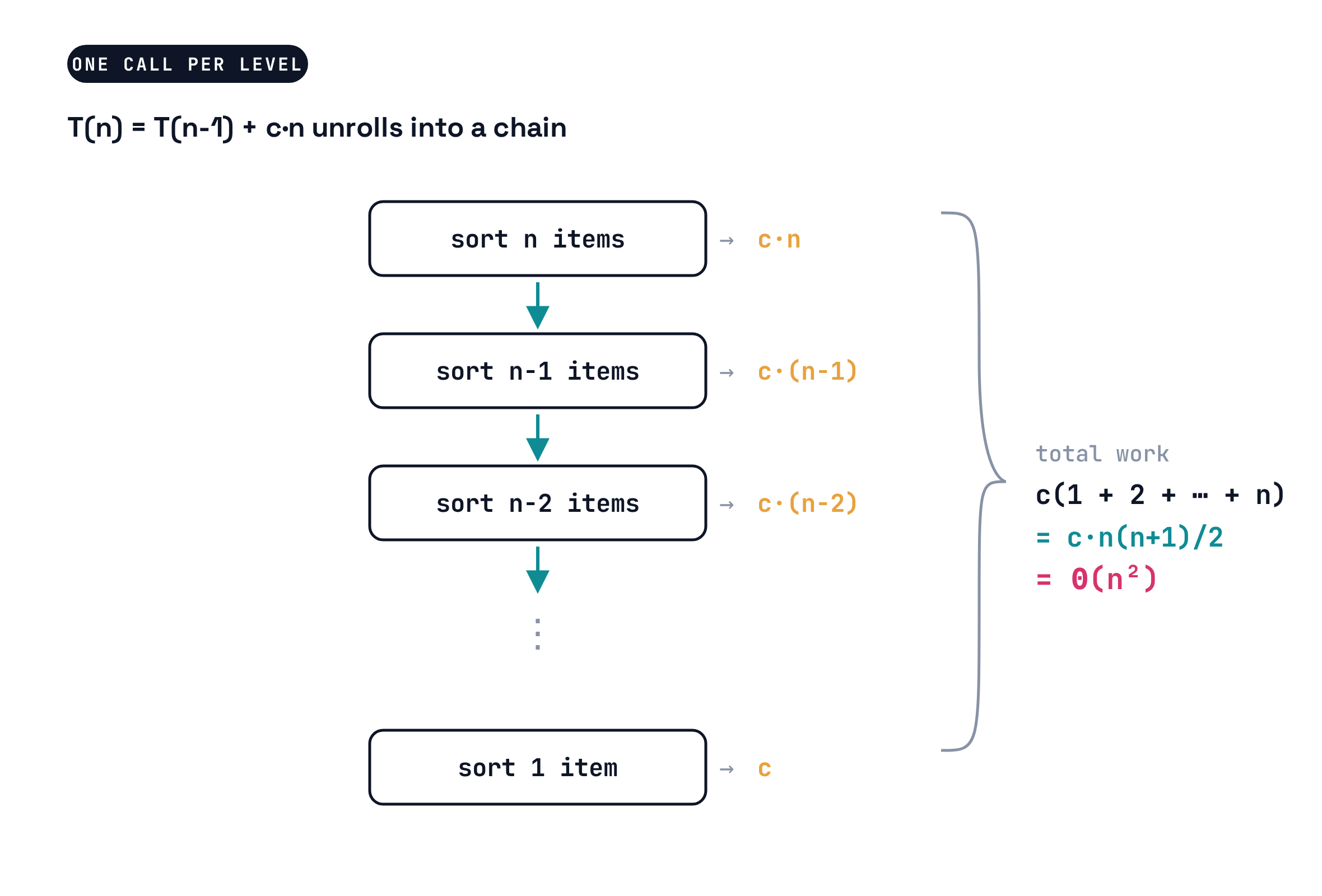
\[T(n) = \underbrace{c \cdot 1 + c \cdot 2 + \cdots + c \cdot (n-1)}_{\text{round } i \text{ costs at most } c \cdot i} = c \cdot \frac{n(n-1)}{2} = \Theta(n^2).\]
The sum, worked out
Round \(i\) inserts key \(A[i]\) into a sorted prefix of length \(i\): at most \(i\) compare-and-swap steps, each costing at most a constant \(c\). The worst case pays full price in every round:
- Add up the rounds: \(T(n) = c + 2c + 3c + \cdots + (n-1)c = c \, \big(1 + 2 + 3 + \cdots + (n-1)\big)\).
- Close the sum by adding it to its own reversal: each of the \(n - 1\) columns of \(\big(1 + \cdots + (n-1)\big) + \big((n-1) + \cdots + 1\big)\) sums to exactly \(n\), so twice the sum is \(n(n-1)\), and \[T(n) = c \cdot \frac{n(n-1)}{2} = \frac{c}{2}\,n^2 - \frac{c}{2}\,n = \Theta(n^2).\]
- Where the two factors of \(n\) come from: one counts the rounds (the chain is \(n\) deep), the other is the width of the later rounds (early keys travel up to \(n\) slots). Depth times typical width.
Sanity check at \(n = 5\): \(T(5) = c(1 + 2 + 3 + 4) = 10c\), and the triangle of work really does hold \(\frac{5 \cdot 4}{2} = 10\) units.
round 1   x
round 2   x x
round 3   x x x
round 4   x x x x
A reverse-sorted input hits every round’s bound, so the worst case really is \(\Theta(n^2)\); an already-sorted input pays one comparison per round, \(\Theta(n)\). The constants \(c\) and \(\tfrac{1}{2}\) vanished into \(\Theta\); the \(n^2\) could not.
Insertion sort’s superpower 💪🏼
- On an already sorted input, every key stops after one comparison: \(\Theta(n)\) total, the best any sort that reads its input can do.
- On a nearly sorted input (each item is at most a few slots from home), it is still \(O(n)\): the cost is \(n\) plus the total distance keys must travel.
- So \(\Theta(n^2)\) is the worst case, not the whole story. Naming which case you are quoting is part of speaking the analysis language correctly.
Remember this superpower for the end of the class; it is why insertion sort never fully retired. 🏝️
Merge sort
Divide and conquer
Insertion sort nibbles: one key per round. Merge sort takes a completely different stance:
- Divide the array into two halves.
- Conquer each half by sorting it recursively; an array of size \(1\) is already sorted.
- Combine the two sorted halves into one sorted array with a merge.
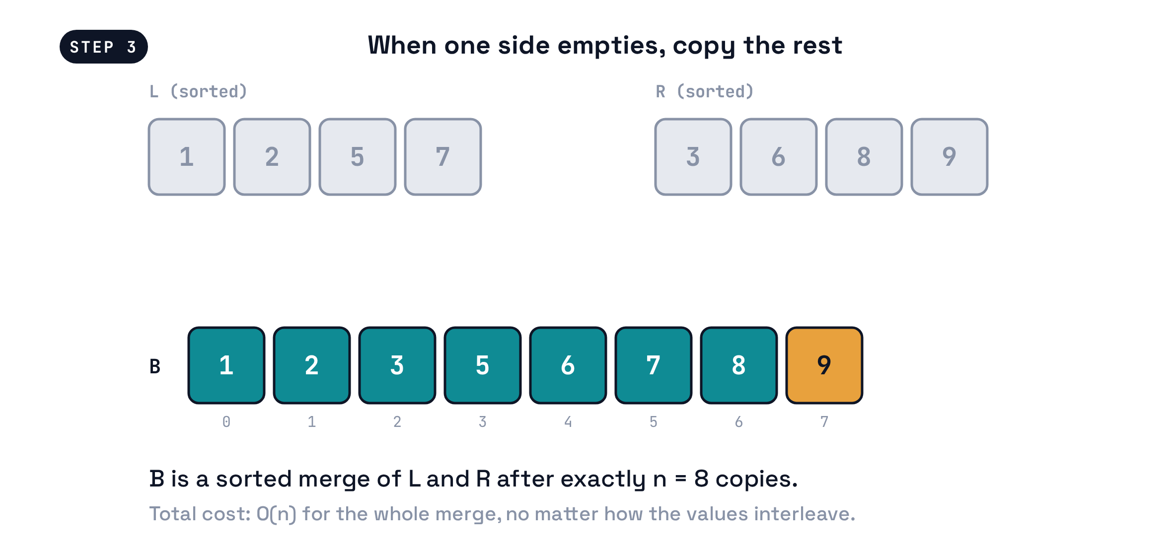
Example: \((5, 2, 7, 1, 9, 3, 8, 6)\) splits into \((5, 2, 7, 1)\) and \((9, 3, 8, 6)\); the recursion hands back \((1, 2, 5, 7)\) and \((3, 6, 8, 9)\); merging gives \((1, 2, 3, 5, 6, 7, 8, 9)\).
All the actual work hides in one question: how cheaply can we merge two sorted arrays?
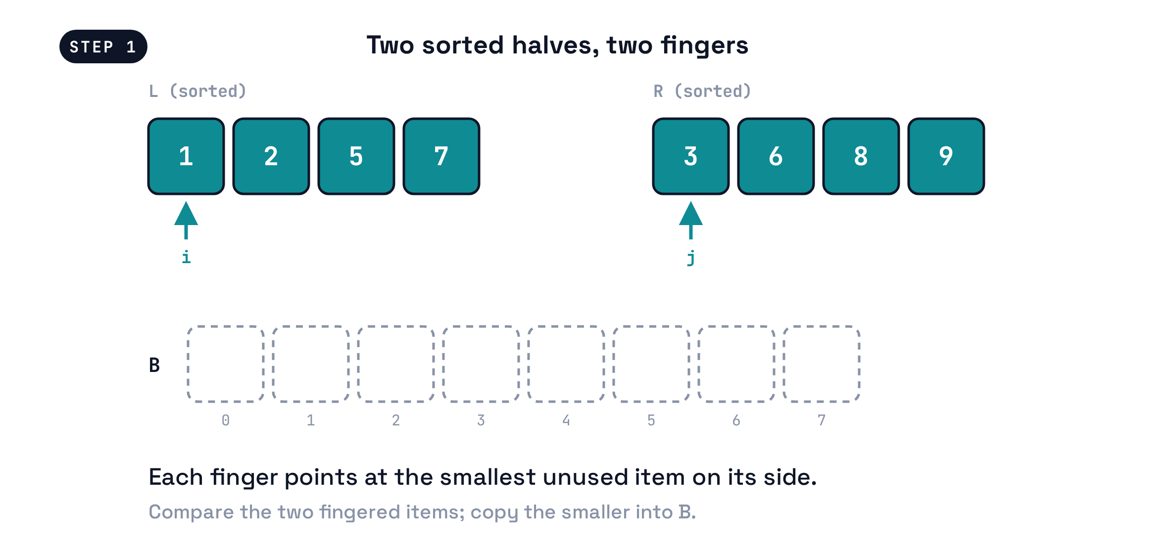
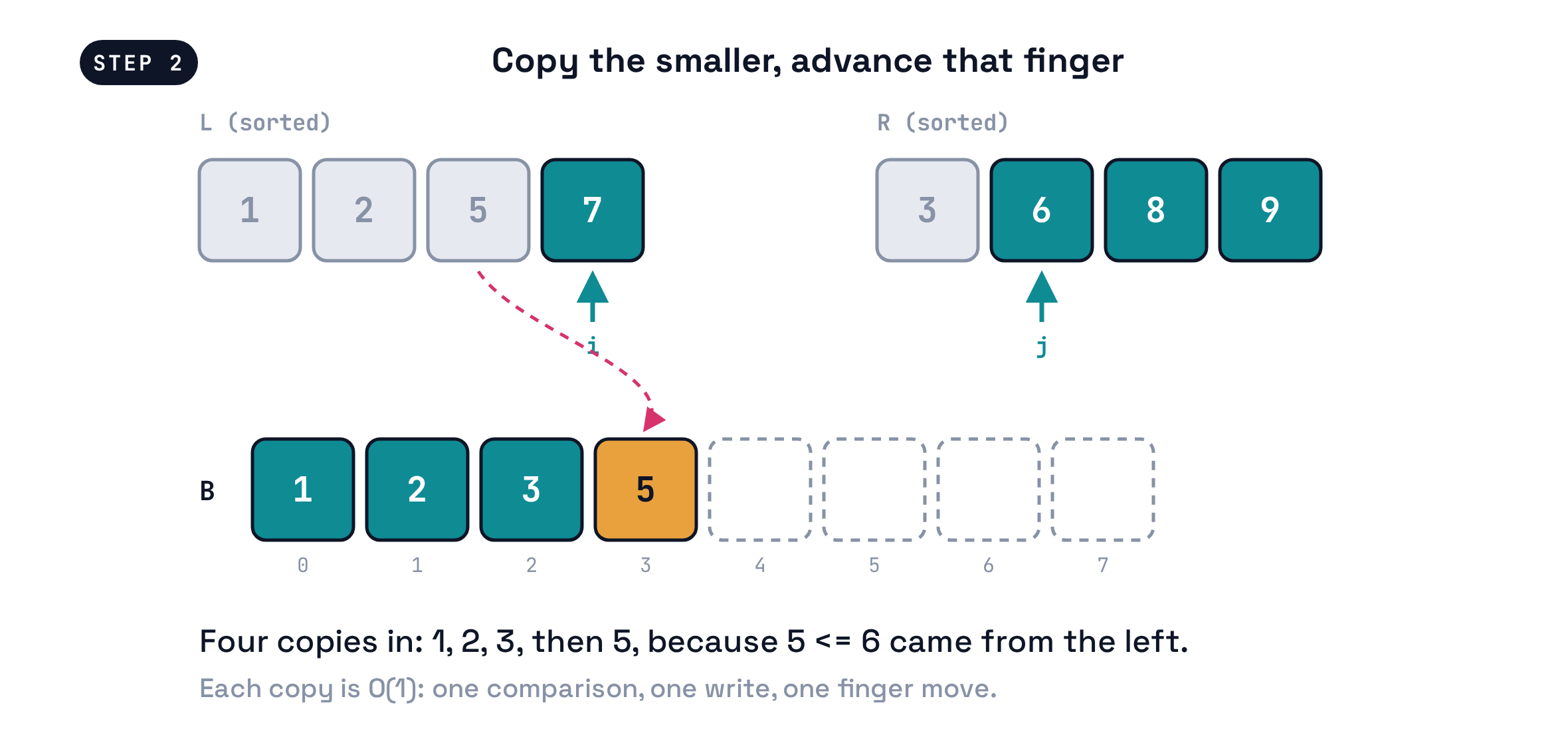
The two-finger merge, frame by frame
The code
def merge_sort(A):                       # T(n)
    if len(A) <= 1:                      # base case: sorted
        return A
    mid = len(A) // 2
    L = merge_sort(A[:mid])              # T(n/2)
    R = merge_sort(A[mid:])              # T(n/2)
    return merge(L, R)                   # O(n)

def merge(L, R):                         # two-finger walk
    B, i, j = [], 0, 0
    while i < len(L) or j < len(R):
        if j >= len(R) or (i < len(L) and L[i] <= R[j]):
            B.append(L[i]); i += 1       # smaller item is at L[i]
        else:
            B.append(R[j]); j += 1       # smaller item is at R[j]
    return B
Why the merge is correct and cheap
- Correct: the smallest item not yet copied must be at one of the two fingers, because \(L\) and \(R\) are each sorted. The merge always copies the smaller fingered item, so \(B\) is filled in increasing order; induction on the number of copies makes this a proof.
- Cheap: every iteration copies exactly one item and never revisits it, so merging \(n\) items costs \(\Theta(n)\), however the values interleave.
- Merge sort is correct by strong induction on \(n\): assume it sorts every array shorter than \(n\); then \(L\) and \(R\) come back sorted, and the merge finishes the job.
Not in place: the merge needs \(\Theta(n)\) extra space for its output. That is part of the price tag we will weigh at the end.
The bill for merge sort
Let \(T(n)\) be the cost of merge sort on \(n\) items. Reading the code:
\[T(1) = c, \qquad T(n) = \underbrace{2 \, T(n/2)}_{\text{two recursive sorts}} + \underbrace{c \cdot n}_{\text{split and merge}}.\]
- For insertion sort, unrolling \(T(n) = T(n-1) + c \cdot n\) gave a chain, and the chain summed to \(\Theta(n^2)\).
- This recurrence branches: each call spawns two smaller calls. Unrolling it gives a tree.
- What does that tree cost in total? You are about to find out by hand.
Activity: build the recursion tree
Your turn, in pairs
Take one worksheet per pair.
Side 1: run merge sort on the array \((6, 2, 8, 4, 7, 1, 5, 3)\): fill in the splitting tree on the way down, then the merged results on the way back up.
Side 2: count the merge work level by level, total it, then generalize from \(n = 8\) to any \(n\).
Finish early? Take on the challenge question at the bottom of side 2.
12 minutes. Worksheets come in at the end; one per pair, both names on it.
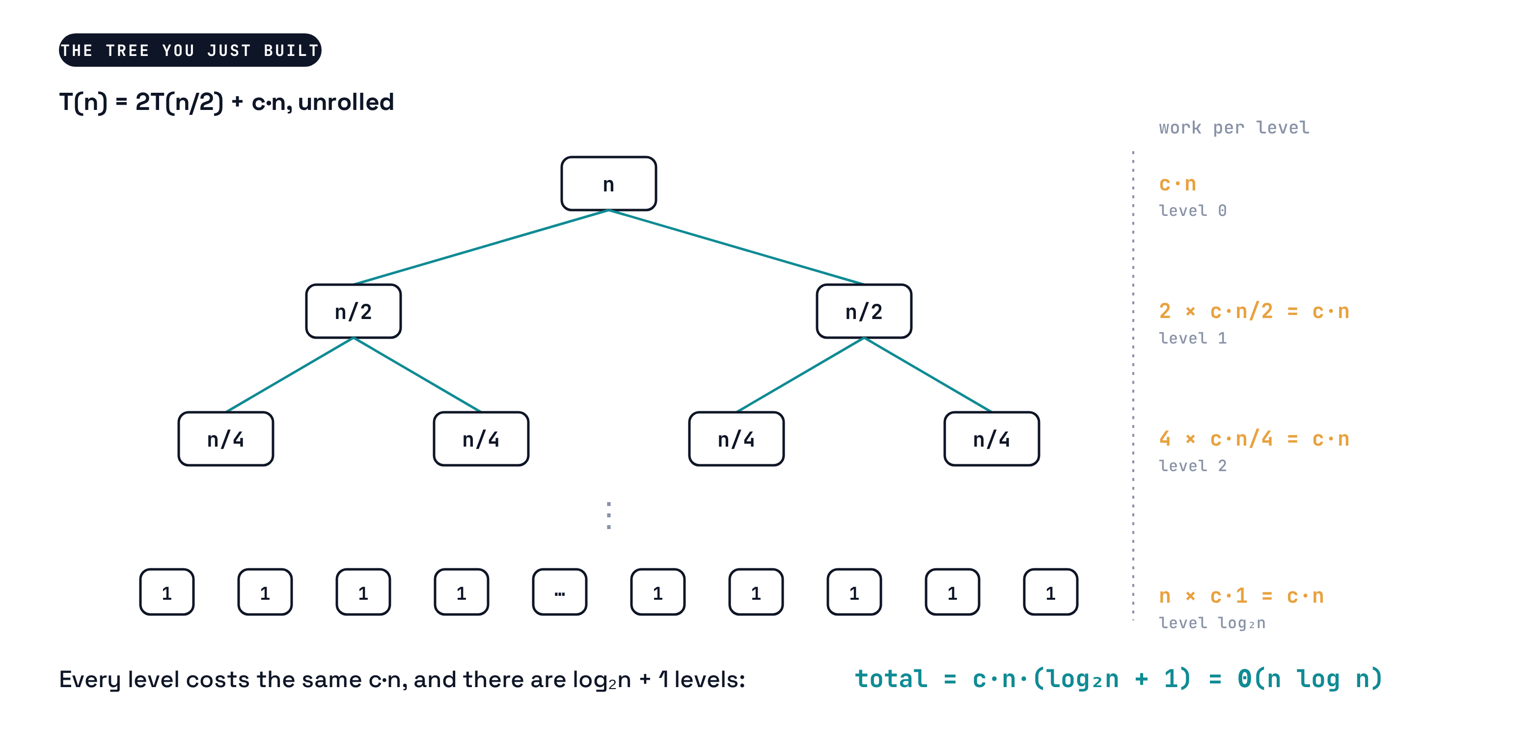
The tree you just built
From the tree to \(n \log n\)
- Level \(i\) of the tree holds \(2^i\) subproblems of size \(n / 2^i\), and merging a level costs \(c \cdot \frac{n}{2^i}\) per node. Multiply: every level costs the same \(2^i \cdot c \cdot \frac{n}{2^i} = c \cdot n\).
- Halving \(n\) down to \(1\) takes \(\log_2 n\) halvings, so the tree has \(\log_2 n + 1\) levels.
- Total: \(c \cdot n \cdot (\log_2 n + 1) = \Theta(n \log n)\), exactly what your worksheet found for \(n = 8\): four levels, \(8c\) each.
Insertion sort’s recurrence unrolled into a chain and cost \(\Theta(n^2)\); merge sort’s unrolled into a balanced tree and cost \(\Theta(n \log n)\). The shape of the recursion decides the bill. On Wednesday we turn this picture into a theorem that solves whole families of recurrences at sight.
The recurrence, worked out
The tree summed the levels for us. Here is the same answer by pure algebra: substitute the recurrence into itself and watch the pattern grow.
- Start with \(T(n) = c\,n + 2\,T(n/2)\) and substitute for \(T(n/2)\): \[T(n) = c\,n + 2\left(c\,\tfrac{n}{2} + 2\,T(n/4)\right) = c\,n + c\,n + 4\,T(n/4).\]
- Each substitution adds one more full \(c\,n\) (twice as many subproblems, each half as big) and doubles the pending calls: after \(k\) rounds, \(T(n) = k \cdot c\,n + 2^k \, T(n/2^k)\).
- The unrolling stops when the subproblems hit size \(1\), at \(2^k = n\), that is \(k = \log_2 n\): \[T(n) = c\,n \log_2 n + n \cdot T(1) = c\,n \log_2 n + c\,n = \Theta(n \log n).\]
Sanity check at \(n = 8\): three levels of merging copy \(8\) items each, \(24\) copies, plus \(8\) base cases: a rectangle of work, \(n\) wide and \(\log_2 n + 1\) tall.
level 0   x x x x x x x x
level 1   x x x x x x x x
level 2   x x x x x x x x
leaves    x x x x x x x x
Triangle versus rectangle is the whole comparison: insertion sort stacks levels of growing width, \(n\) of them; merge sort stacks levels of constant width, only \(\log_2 n + 1\) of them.
Which sort, when
The sorting scorecard
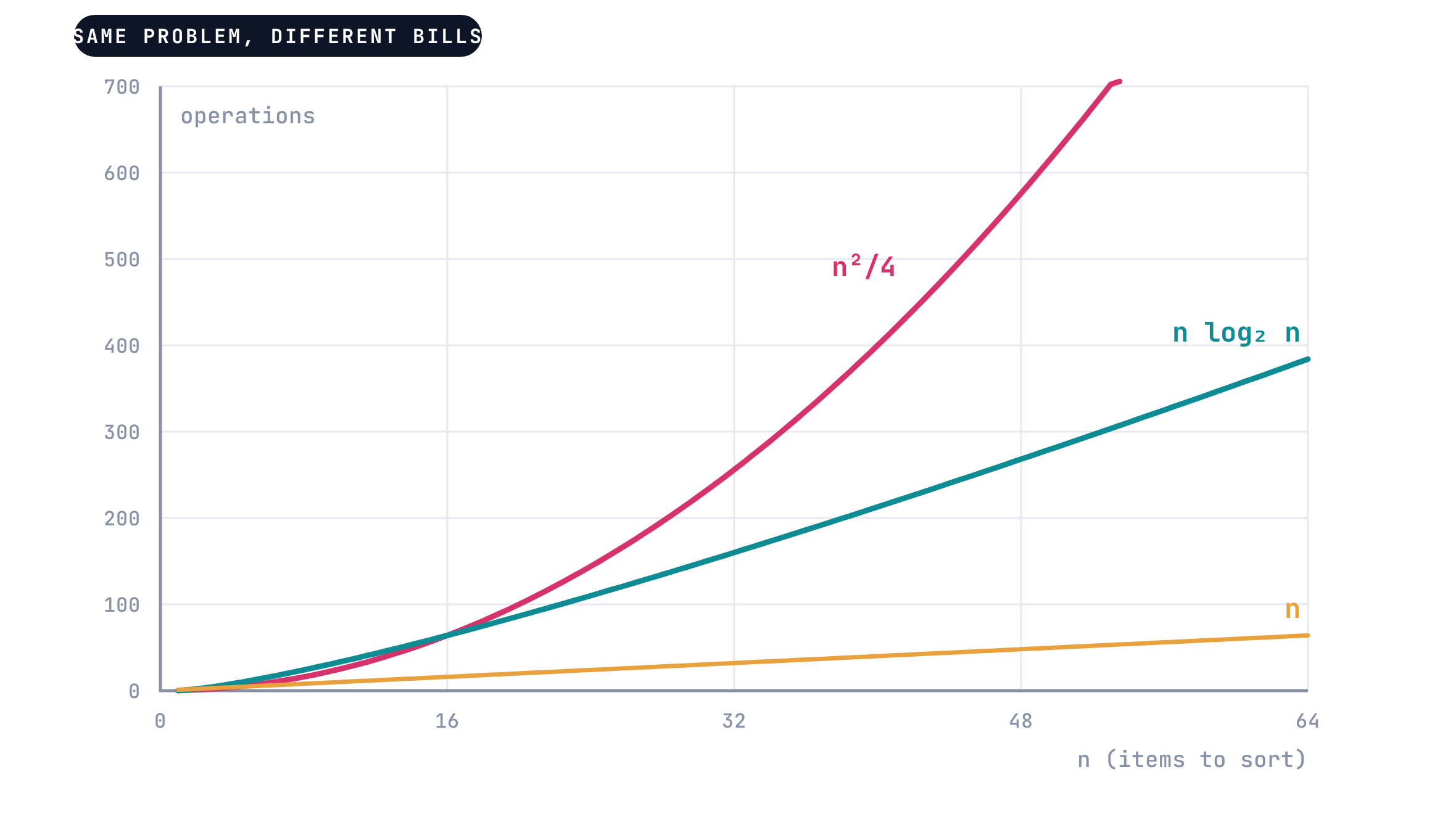
| Algorithm | Worst case | Sorted input | Extra space | In place? |
|---|---|---|---|---|
| Permutation sort | \(\Omega(n! \cdot n)\) | \(O(n)\) | \(O(n)\) | no |
| Insertion sort | \(\Theta(n^2)\) | \(\Theta(n)\) | \(O(1)\) | yes |
| Merge sort | \(\Theta(n \log n)\) | \(\Theta(n \log n)\) | \(O(n)\) | no |
Reading the scorecard like an algorithm pro
- At \(n = 10^6\): roughly \(10^{12}\) steps for insertion sort versus \(2 \times 10^7\) for merge sort. That is the difference between hours and a blink.
- But for small arrays (a few dozen items) or nearly sorted ones, insertion sort’s low overhead and \(O(n)\) best case win the race.
- Real libraries split the difference: Python’s
sortedandlist.sortuse Timsort, which merges sorted runs and hands small pieces to an insertion-style sort. Both of today’s algorithms are inside every Python program you have ever run.
Same lesson as Wednesday’s data structures: there is no best sort, only a best sort for a workload. The analysis is what lets you name which.
Wrap-up
The one-slide version
Sorting is a problem; algorithms are bids to solve it. Brute force is correct and unaffordable. Insertion sort grows a sorted prefix: an induction proof, \(\Theta(n^2)\) worst case, unbeatable on nearly sorted input. Merge sort divides, recurses, and merges with two fingers: \(\Theta(n \log n)\) always, paid for with \(\Theta(n)\) extra space. And recursion trees turn recurrences into pictures you can total up.
What’s next
Wednesday at a glance
Topics: Divide and conquer as a design pattern, and recurrences as its price tags: recursion trees in general, and the Master Theorem, which solves \(T(n) = a\,T(n/b) + f(n)\) on sight.
Supplemental reading (highly recommended): CLRS Chapter 4, in your own copy or online through Canvas/Perusall.
Upcoming deliverables:
- HW0 due tonight at 9:59 PM, via Canvas.
- HW1 due Wednesday, September 9 at 9:59 PM, via Canvas.
References
Sources
- Cormen, T. H., Leiserson, C. E., Rivest, R. L., and Stein, C. Introduction to Algorithms, 4th edition, MIT Press. Chapter 2; Section 4.4.