Divide and Conquer

Lecture W2W1: Recurrences, Recursion Trees, and the Master Theorem

Lucas P. Cordova, Ph.D.

lpcordova@willamette.edu

Willamette University

September 2, 2026

Before we begin: announcements

Three things worth knowing

Our class Discord server has launched. The invite link is in the Quick Links on the Canvas home page. Announcements, questions, and study coordination all live there; come say hello.
No class Monday (Labor Day). Enjoy the long weekend.
Next Wednesday, September 9, I will be away, and Sam will be teaching the class. Be nice to him.

And a reminder: HW1 is due Wednesday, September 9 at 9:59 PM. Everything on it is covered by the end of today.

Learning objectives

What you will leave with

By the end of today, you will be able to:

Recognize the divide-and-conquer pattern and write down the recurrence that it produces.
Build the recursion tree for any such recurrence and identify its pattern: root-dominated, balanced, or leaf-dominated.
Compute the watershed function and explain why it counts the leaves.
Apply the Master Theorem to solve recurrences on sight, and detect when it does not apply.
Explain how Strassen’s algorithm multiplies matrices faster.

Recap of Monday

Monday’s class in four bullets:

Sorting is a problem; algorithms are ways to solve it. Brute force (permutation sort) is correct but expensive, which is why analysis exists.
Insertion sort grows a sorted prefix one key at a time. Worst case, the rounds cost \(1, 2, \ldots\) up to \(n\) units: we claimed \(\Theta(n^2)\).
Merge sort splits in half, sorts each half, and merges with two fingers. Your recursion-tree activity found every level costs the same, and read off \(\Theta(n \log n)\).
Both totals came from pictures: a triangle of work and a rectangle of work.

Today’s goal

Go over the math behind the last class then meet a theorem that skips the algebra entirely, and spend the rest of class learning to apply it fast.

The math behind Monday

Exponents in one minute

\(a^k\) means \(k\) copies of \(a\) multiplied together: \(2^3 = 2 \cdot 2 \cdot 2 = 8\). Every rule below is just counting copies:

\(a^m \cdot a^n = a^{m+n}\) \(m\) copies times \(n\) more copies is \(m + n\) copies
\(\dfrac{a^m}{a^n} = a^{m-n}\) \(n\) of the copies cancel top and bottom
\((a^m)^n = a^{m \cdot n}\) \(n\) groups of \(m\) copies each
\(\left(\dfrac{a}{b}\right)^{k} = \dfrac{a^k}{b^k}\) each copy of the fraction puts one \(a\) on top and one \(b\) below
\(a^0 = 1\) zero copies: nothing multiplied yet, so the running product is still 1

Logarithms in one minute

\(\log_b n\) answers exactly one question: how many times must I multiply by \(b\) to reach \(n\)?

\(\log_2 8 = 3\) because \(2 \cdot 2 \cdot 2 = 8\): three doublings reach 8
\(b^{\log_b n} = n\) the same sentence written as an equation: multiply \(b\) by itself “that many” times and you land on \(n\)
Read backwards, \(\log_b n\) is also how many times you can divide \(n\) by \(b\) before hitting 1 the same ladder, climbed down instead of up
The backwards reading is why logs fill this course: halving \(n\) down to \(1\) takes exactly \(\log_2 n\) halvings, so every halving recursion is \(\log_2 n\) levels deep.

Check: \(n = 16 \to 8 \to 4 \to 2 \to 1\) is four halvings, and \(\log_2 16 = 4\).

Gauss’s beautiful trick

The story: a schoolteacher assigns young Gauss \(1 + 2 + \cdots + 100\) as busywork; he answers \(5050\) in seconds. His idea: do not add left to right; pair the ends.

\(1 + 100 = 101\), and \(2 + 99 = 101\), and \(3 + 98 = 101\): every pair, working inward, is worth \(101\). Fifty pairs: \(50 \cdot 101 = 5050\).
The general version arranges the numbers in two rows: the sum \(S\) written forward, then the same sum written backward. \[\begin{array}{cccccc} 1 & 2 & 3 & \cdots & n-1 & n\\ n & n-1 & n-2 & \cdots & 2 & 1 \end{array}\]
A row is read horizontally: each row is one full copy of \(S\). A column is read vertically: each column pairs one small number with one large one.

Why every column is worth the same

\[\begin{array}{cccccc} 1 & 2 & 3 & \cdots & n-1 & n\\ n & n-1 & n-2 & \cdots & 2 & 1 \end{array}\]

Look at the column in position \(k\), counting from the left:

Its top entry is \(k\). row 1 counts up from 1, so position \(k\) holds \(k\)
Its bottom entry is \(n - k + 1\). row 2 counts down from \(n\): position 1 holds \(n\), position 2 holds \(n-1\), and so on
Column total: \(k + (n - k + 1) = n + 1\). the \(k\) cancels: whatever the top gains by being further right, the bottom loses
The position \(k\) dropped out of the answer. So every column totals the same \(n + 1\), no matter which column you pick. That cancellation is the entire trick.

Check it at \(n = 5\): the columns are \((1,5),\,(2,4),\,(3,3),\,(4,2),\,(5,1)\), and every one of them totals \(6\).

Counting the same pile two ways

Every number in the table gets added exactly once either way, so the two grand totals must agree:

By rows: each row is one full copy of \(S\), so the grand total is \(S + S = 2S\). true, but useless by itself: we do not know \(S\) yet
By columns: there are \(n\) columns, each worth \(n+1\). Adding \(n\) copies of the same number is exactly what multiplication is, so the grand total is \(n \cdot (n+1)\). this one we can actually compute
Same numbers, same total: \(2S = n(n+1)\), so \(S = \dfrac{n(n+1)}{2}\).

Check at \(n = 5\): by rows, \(15 + 15 = 30\); by columns, \(5 \cdot 6 = 30\). So \(2S = 30\) and \(S = 15\), which is indeed \(1+2+3+4+5\).

Gauss, in one line

Whenever you meet \(1 + 2 + \cdots + n\), its value is \(\frac{n(n+1)}{2}\): roughly half of \(n^2\). (\(n(n+1)\) is the area of an \(n \times (n+1)\) rectangle, and two staircase copies of \(S\), one flipped upside down, tile it exactly.) That is the only fact insertion sort’s bill needs.

Insertion sort’s bill, line by line

Monday’s chain, turned into algebra. Each line does one thing:

\(T(n) = c\,n + c\,(n-1) + \cdots + c \cdot 2 + c \cdot 1\) unroll the chain: the first call does \(c\,n\) work, the next \(c\,(n-1)\), down to \(c\)
\(T(n) = c\,\big(n + (n-1) + \cdots + 2 + 1\big)\) every term shares a factor of \(c\); factor it out
\(T(n) = c \cdot \dfrac{n(n+1)}{2}\) the parenthesis is exactly Gauss’s sum from the last slide
\(T(n) = \dfrac{c}{2}\,n^2 + \dfrac{c}{2}\,n\) multiply out: \(n(n+1) = n^2 + n\)
\(T(n) = \Theta(n^2)\) as \(n\) grows, the \(n^2\) term dwarfs the \(n\) term; \(\Theta\) keeps the leader and drops constants

Sanity check with real numbers: \(n = 4\) gives \(c(4 + 3 + 2 + 1) = 10c\), and the formula gives \(c \cdot \frac{4 \cdot 5}{2} = 10c\). They agree, so trust the letters.

Merge sort’s bill: a different kind of problem

Insertion sort handed us a finished list of numbers to add, \(1 + 2 + \cdots + n\), and Gauss’s pairing trick added it. Merge sort hands us something else entirely:

\(T(n) = c\,n + 2\,T\!\left(\tfrac{n}{2}\right)\) is a rule, not a list: “the bill for size \(n\) is \(c\,n\) for the split and merge, plus two more bills for size \(n/2\).” and each of those bills contains two more bills, and so on
We cannot pair anything yet, because there is no list of numbers to pair. First we must chase the rule down until it stops producing new bills.
The tool for that is substitution: the rule holds at every size, so the rule itself tells us what \(T(n/2)\) is. Feed the rule into itself, one layer at a time.

So this is a genuinely different kind of solve from Gauss. It will end in a sum too, but a much friendlier one: the layers will all turn out to be identical, so no pairing trick is needed at all.

Merge sort’s bill: unroll the recurrence

Feed the rule into itself, watching what each substitution does:

\(T(n) = c\,n + 2\,T\!\left(\tfrac{n}{2}\right)\) the recurrence itself
\(T(n) = c\,n + 2\left[c\,\tfrac{n}{2} + 2\,T\!\left(\tfrac{n}{4}\right)\right]\) replace \(T(n/2)\) with what the recurrence says at size \(n/2\)
\(T(n) = c\,n + c\,n + 4\,T\!\left(\tfrac{n}{4}\right)\) multiply through: \(2 \cdot c\,\tfrac{n}{2} = c\,n\), and \(2 \cdot 2 = 4\) quarter-size sorts
\(T(n) = c\,n + c\,n + c\,n + 8\,T\!\left(\tfrac{n}{8}\right)\) substitute again: \(4 \cdot c\,\tfrac{n}{4}\) is yet another \(c\,n\)
\(T(n) = k \cdot c\,n + 2^k\,T\!\left(\tfrac{n}{2^k}\right)\) the pattern after \(k\) substitutions: \(k\) full copies of \(c\,n\), plus \(2^k\) small sorts still pending

Why every substitution adds exactly \(c\,n\): at step \(i\) there are \(2^i\) pending sorts of size \(n/2^i\), and \(2^i \cdot c \cdot \frac{n}{2^i} = c\,n\). Twice as many pieces, each half as big: the two effects cancel perfectly. the layer number cancels here, the way the position \(k\) cancelled for Gauss

Merge sort’s bill: stop the machine

The substitutions stop when the pending sorts hit arrays of size 1, which are already sorted:

\(\dfrac{n}{2^k} = 1\), that is, \(2^k = n\) the stopping condition: \(k\) halvings have taken \(n\) all the way down to 1
\(k = \log_2 n\) that is the definition of the logarithm from three slides ago
\(T(n) = c\,n \log_2 n + n \cdot T(1)\) plug \(k = \log_2 n\) into the pattern; \(2^k = n\) base cases remain
\(T(n) = c\,n \log_2 n + c\,n\) each size-1 base case costs a constant, \(T(1) = c\)
\(T(n) = \Theta(n \log n)\) the lone \(c\,n\) grows slower than \(c\,n \log_2 n\); \(\Theta\) keeps the leader

Sanity check: \(n = 8\) gives \(8 \cdot 3 + 8 = 32\), and Monday’s worksheet counted \(24\) merge copies plus \(8\) base cases. They agree.

Two sums, two solves

Notice where each sum got easy:

	Insertion sort	Merge sort
What we had to add	layers of different sizes: \(1, 2, \ldots, n\)	layers of identical size: \(c\,n\) each
How many layers	\(n\)	\(\log_2 n\)
How to add them	Gauss’s pairing trick	just count: \(\log_2 n\) layers \(\times\) \(c\,n\)
The bill	\(\Theta(n^2)\)	\(\Theta(n \log n)\)

Why we need a theorem

We just spent five lines of algebra on one recurrence, and dozens more are coming this semester. The Master Theorem answers them in one step. Learning to use it is the rest of today.

The divide-and-conquer pattern

Three verbs

Merge sort was not a one-off. It is an instance of a design pattern:

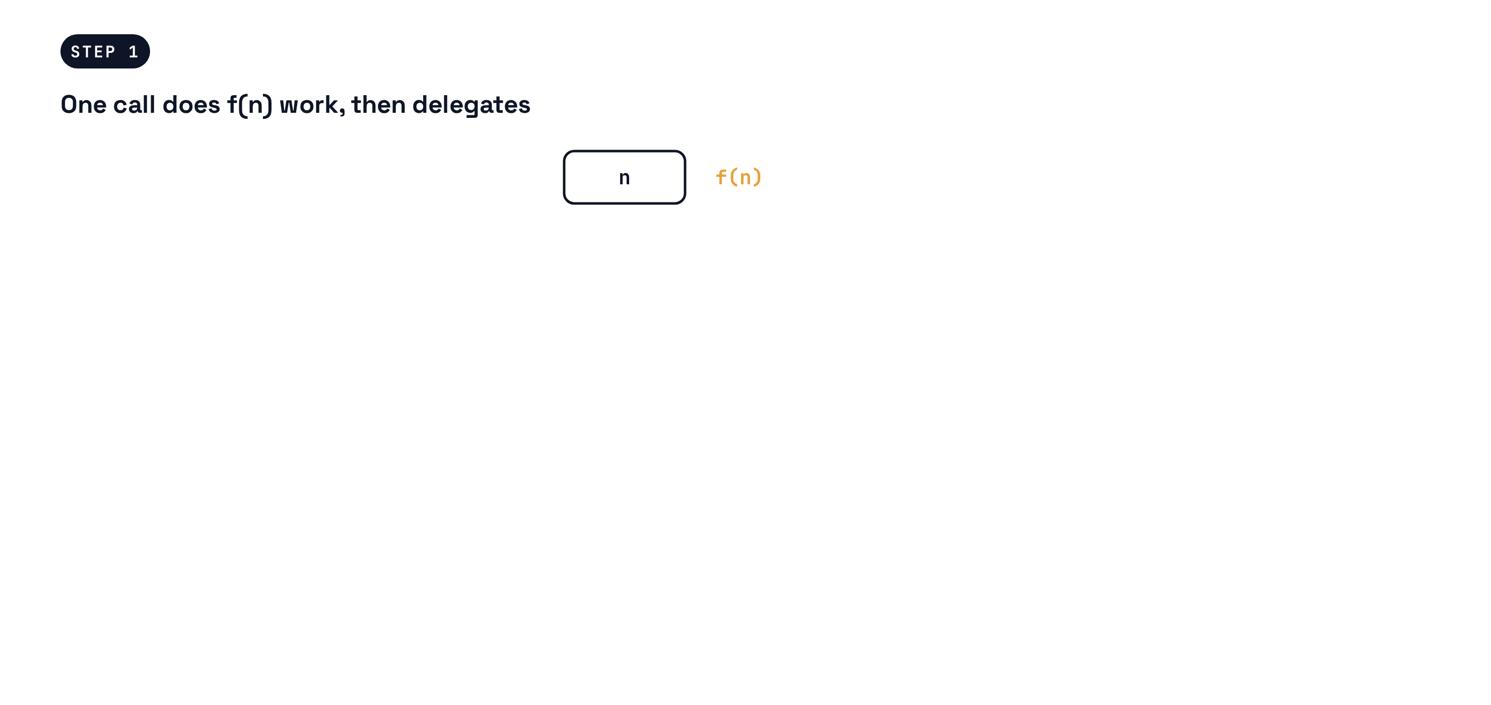
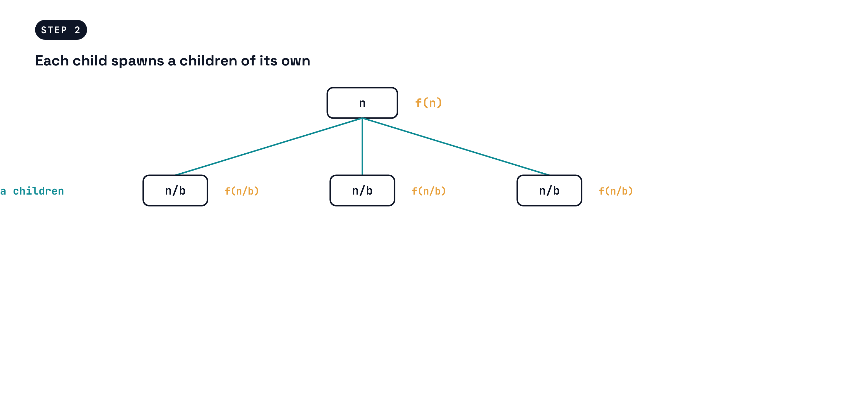
Divide the problem into \(a\) subproblems, each of size \(n/b\).
Conquer each subproblem recursively; solve constant-size problems directly.
Combine the subproblem answers into the answer for the whole, spending \(f(n)\) work on the divide and combine steps together.

For merge sort: \(a = 2\) subproblems, each \(b = 2\) times smaller, and the split plus the two-finger merge cost \(f(n) = \Theta(n)\).

The pattern’s price tag

Every algorithm built this way has running time \(T(n) = a \, T(n/b) + f(n)\). Analyze the pattern once, and you have analyzed every algorithm that will ever fit it.

You already know another one

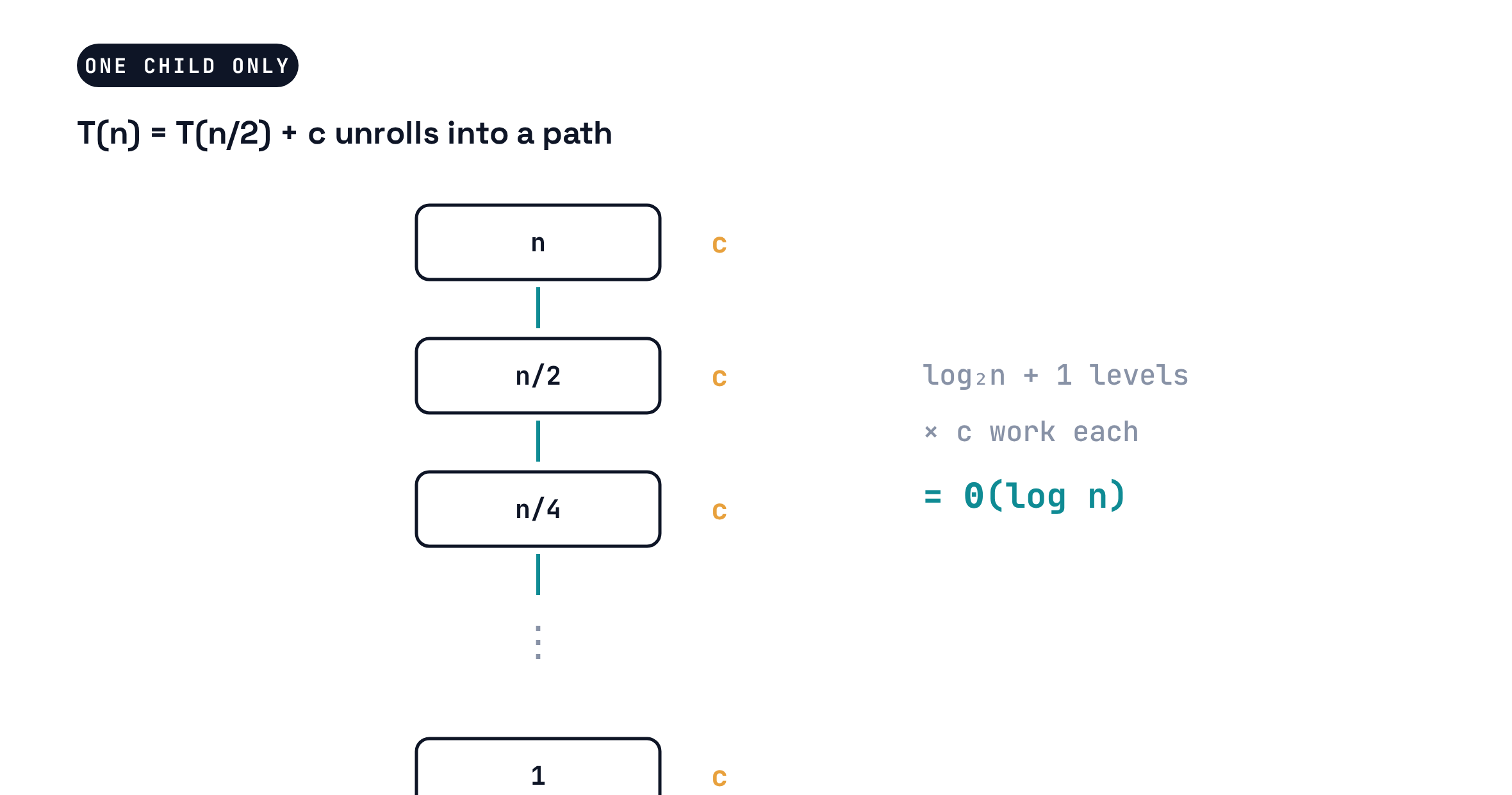
Binary search fits the pattern with the smallest possible numbers: to find key \(k\) in a sorted array, compare against the middle and recurse on one half.

\[T(n) = 1 \cdot T(n/2) + c \qquad (a = 1, \; b = 2, \; f(n) = c)\]

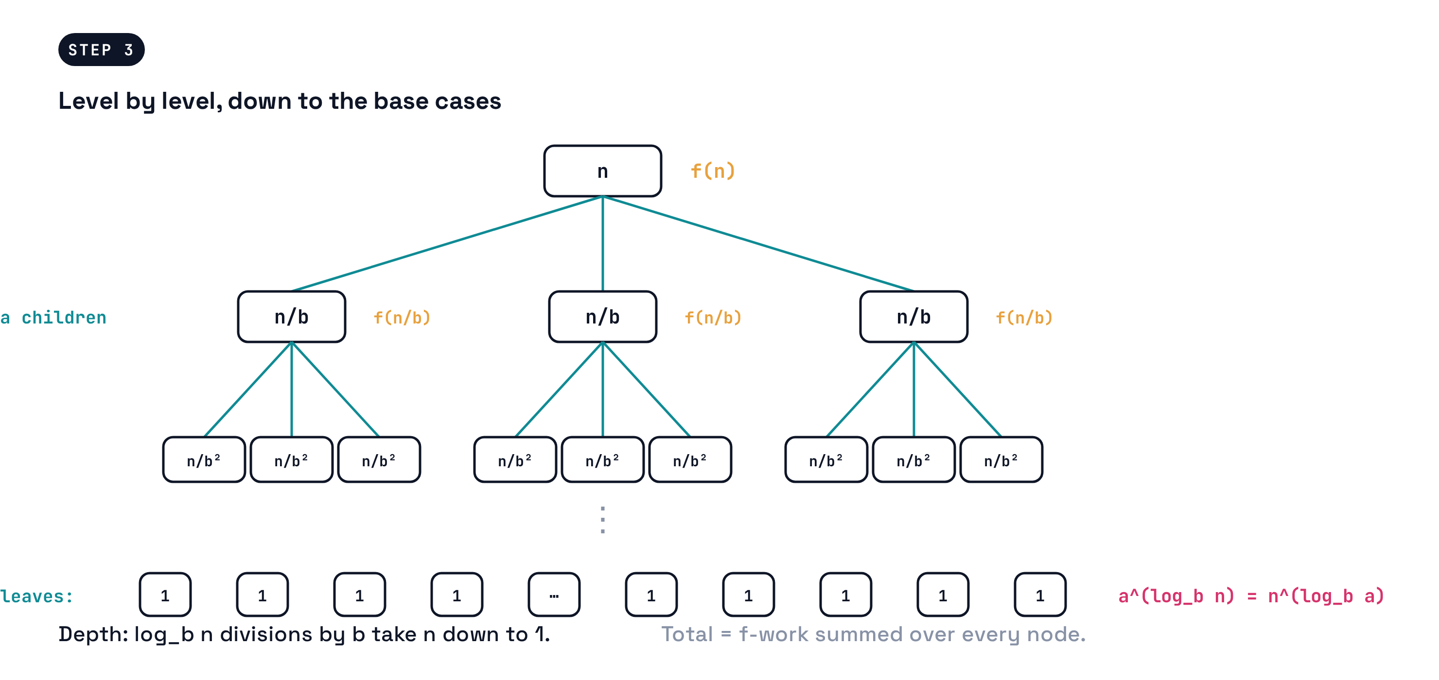
The tree, in general

The watershed function: counting the leaves

How many leaves does the tree of \(T(n) = a\,T(n/b) + f(n)\) have?

The tree is \(\log_b n\) levels deep: that is how many times you can divide \(n\) by \(b\) before hitting \(1\).
Each level multiplies the node count by \(a\), so the leaf count is \(a^{\log_b n}\).
A logarithm identity turns that inside out: \(a^{\log_b n} = n^{\log_b a}\). Check it on merge sort: \(a = b = 2\) gives \(n^{\log_2 2} = n\) leaves, one per item. Correct.

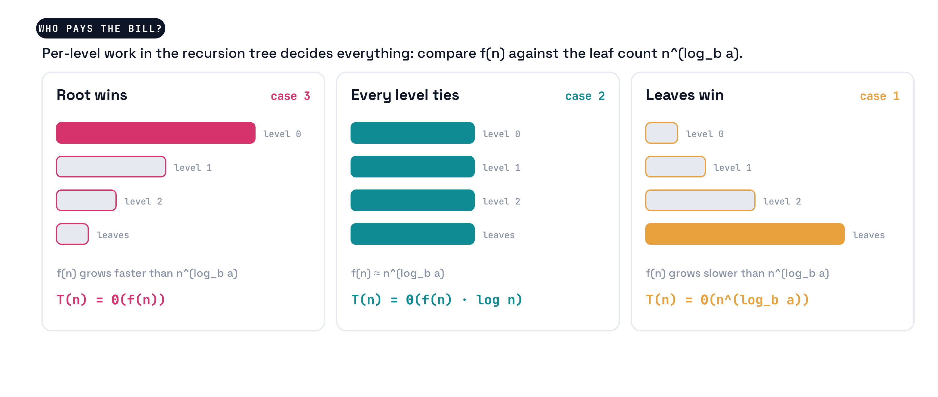
\(n^{\log_b a}\) is the watershed function: the total cost of the bottom of the tree. The whole analysis reduces to one question: does \(f(n)\) grow faster, slower, or at the same rate as \(n^{\log_b a}\)?

Why “watershed”? A watershed is the ridge line on a mountain range: rain that lands on one side flows to one river, rain on the other side flows to the other. \(n^{\log_b a}\) is the ridge.

The watershed, pictured

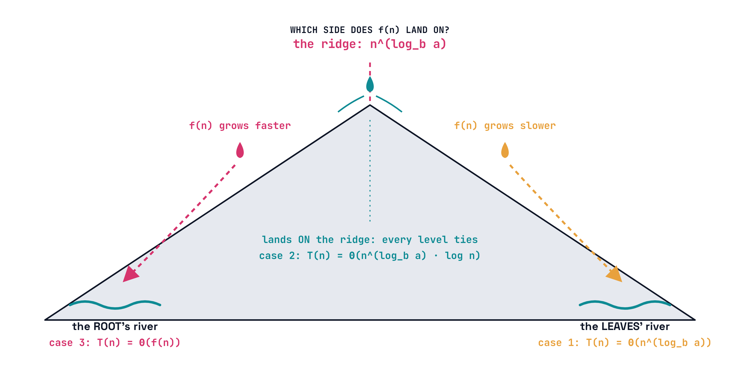
A course nickname, not standard notation: CLRS just writes \(n^{\log_b a}\).

The three regimes

Who pays the bill?

The cast of characters

Before the theorem, the four symbols in \(T(n) = a\,T(n/b) + f(n)\), in plain words:

Symbol	Meaning
\(a\)	how many subproblems each call spawns
\(b\)	how many times smaller each subproblem is than its parent
\(f(n)\)	the work a call does itself: dividing and combining
\(n^{\log_b a}\)	the watershed: the total cost of all the leaves

Read the first three straight off the recurrence; compute the fourth. Same four every time, for every divide-and-conquer algorithm you will ever meet.

The Master Theorem

Master Theorem. Let \(T(n) = a\,T(n/b) + f(n)\) with \(a \geq 1\) and \(b > 1\) constants. Compare \(f(n)\) to \(n^{\log_b a}\):

Leaves win. If \(f(n) = O(n^{\log_b a - \varepsilon})\) for some \(\varepsilon > 0\), then \(T(n) = \Theta(n^{\log_b a})\).
Tie. If \(f(n) = \Theta(n^{\log_b a} \log^k n)\) for some \(k \geq 0\), then \(T(n) = \Theta(n^{\log_b a} \log^{k+1} n)\).
Root wins. If \(f(n) = \Omega(n^{\log_b a + \varepsilon})\) for some \(\varepsilon > 0\) (plus a mild regularity condition that everything in this course satisfies), then \(T(n) = \Theta(f(n))\).

It is not magic: each case is exactly one of the three tree shapes, with the geometric series summed once and for all. The theorem is Monday’s activity, industrialized.

Reading it like a practitioner

The same three moves, every single time: (1) read \(a\), \(b\), and \(f(n)\) straight off the recurrence, (2) compute the watershed \(n^{\log_b a}\), (3) compare \(f(n)\) against it and name the case. Three examples, solved at sight:

Merge sort, \(T(n) = 2\,T(n/2) + \Theta(n)\): watershed \(n^{\log_2 2} = n\), and \(f(n) = \Theta(n)\) ties it (case 2, \(k = 0\)): \(T(n) = \Theta(n \log n)\). Matches Monday.
Binary search, \(T(n) = T(n/2) + \Theta(1)\): watershed \(n^{\log_2 1} = n^0 = 1\), and \(f(n) = \Theta(1)\) ties it (case 2, \(k = 0\)): \(T(n) = \Theta(\log n)\). Matches the path picture.
Blocked matrix multiply, \(T(n) = 8\,T(n/2) + \Theta(n^2)\): watershed \(n^{\log_2 8} = n^3\), and \(n^2\) grows slower (case 1): \(T(n) = \Theta(n^3)\). Hold this thought for the end of class.

The fine print

The theorem is powerful, but it cannot digest every recurrence. It stays silent when:

The recurrence has the wrong shape. \(T(n) = T(n - 1) + c \cdot n\) shrinks by subtraction, not division: there is no \(b > 1\). Recursion tree (a chain) still works: \(\Theta(n^2)\).
\(f(n)\) falls between the cases. For \(T(n) = 2\,T(n/2) + n / \log n\), \(f\) is smaller than \(n\) but not polynomially smaller: no \(\varepsilon\) works. The tree still works; the theorem as stated does not.
The subproblems have unequal sizes. \(T(n) = T(n/3) + T(2n/3) + c \cdot n\) is real divide and conquer, but not \(a\) copies of \(n/b\). (A recursion tree handles it; the level costs stay \(\Theta(n)\) for \(\Theta(\log n)\) levels.)

When in doubt, draw the tree

The Master Theorem is a compiled recursion tree. When it does not apply, do not force it; draw the tree.

Activity: the Master Method clinic

Your turn, in pairs

Take one worksheet per pair. Eight recurrences have come to the clinic complaining about their running times.

Side 1: for each patient, chart \(a\), \(b\), the watershed \(n^{\log_b a}\), the case, and the \(\Theta\) diagnosis. Warning: not every patient can be treated by the Master Theorem; write “refer out” and say why.

Side 2: two published “proofs” contain malpractice; find the flaw in each. Then design your own patient with a prescribed diagnosis.

10 minutes. Worksheets come in at the end; one per pair, both names on it.

Clinic debrief

Patient	\(n^{\log_b a}\)	Case	Diagnosis
\(2T(n/2) + c\,n\)	\(n\)	2	\(\Theta(n \log n)\)
\(9T(n/3) + c\,n\)	\(n^2\)	1	\(\Theta(n^2)\)
\(T(n/2) + c\)	\(1\)	2	\(\Theta(\log n)\)
\(3T(n/3) + c\,n^2\)	\(n\)	3	\(\Theta(n^2)\)
\(8T(n/2) + c\,n^2\)	\(n^3\)	1	\(\Theta(n^3)\)
\(7T(n/2) + c\,n^2\)	\(n^{\log_2 7}\)	1	\(\Theta(n^{\log_2 7})\)
\(2T(n/2) + c\,n \log n\)	\(n\)	2, \(k=1\)	\(\Theta(n \log^2 n)\)
\(T(n-1) + c\,n\)	refer out		\(\Theta(n^2)\) by chain

The last row is the trap that matters most in practice: check the shape before you reach for the theorem.

The payoff: multiplying matrices

Eight multiplications… or seven

Multiplying two \(n \times n\) matrices the definitional way costs \(\Theta(n^3)\). Divide and conquer seems to offer hope: split each matrix into four \(\frac{n}{2} \times \frac{n}{2}\) blocks.

The block formula needs \(a = 8\) block products of size \(n/2\), plus \(\Theta(n^2)\) of block additions: \(T(n) = 8\,T(n/2) + \Theta(n^2) = \Theta(n^3)\). No progress: the leaves win, and there are just as many.
In 1969, Volker Strassen found seven cleverly chosen block products whose sums and differences reconstruct all four blocks of the answer: \(a\) drops from \(8\) to \(7\).
\(T(n) = 7\,T(n/2) + \Theta(n^2) = \Theta(n^{\log_2 7}) = \Theta(n^{2.81})\). The exponent moved.

Where the money is

\(f(n)\) was untouched; shrinking \(a\) rewrote the watershed. In a leaf-dominated recurrence, the branching factor is where the money is.

How low can the exponent go?

Strassen’s \(n^{2.81}\) is not the end: decades of research have pushed the exponent below \(2.38\), though the record-holders have constants so large they are impractical, a reminder from Monday that constants are real.
Nobody knows the true limit. The conjecture many believe: matrix multiplication in \(n^{2 + \varepsilon}\) for every \(\varepsilon > 0\). Proving or refuting it is one of the great open problems of the field.
What you should take from it: the Master Theorem is not just a homework tool. Reading a recurrence tells you where an algorithm can be improved. Strassen read case 1 and attacked \(a\).

Wrap-up

The one-slide version

Divide and conquer always bills you \(T(n) = a\,T(n/b) + f(n)\). Its recursion tree has three possible shapes: root-heavy, balanced, or leaf-heavy, and the watershed \(n^{\log_b a}\), the cost of the leaves, tells you which by one comparison against \(f(n)\). The Master Theorem is that comparison, precomputed. When the recurrence has the wrong shape, draw the tree instead. And when the leaves win, improving the algorithm means attacking \(a\): that is how matrix multiplication got faster.

What’s next

Week 3 at a glance

No class Monday (Labor Day). We meet again Wednesday, September 9, when Sam takes the wheel.

Topics for Wednesday: Hashing: how dictionaries answer find(k) in constant expected time, without sorting anything. A third notion of cost, expected time, joins worst-case and amortized.

Supplemental reading (highly recommended): CLRS Chapter 11.

Upcoming deliverables:

HW1 due Wednesday, September 9 at 9:59 PM.
HW2 assigned Wednesday, September 9.

References

Sources

Cormen, T. H., Leiserson, C. E., Rivest, R. L., and Stein, C. Introduction to Algorithms, 4th edition, MIT Press. Chapter 4.
Strassen, V. (1969). Gaussian elimination is not optimal. Numerische Mathematik, 13, 354-356.