Hashing

Lecture W3W1: Dictionaries in Constant Expected Time

Lucas P. Cordova, Ph.D.

lpcordova@willamette.edu

Willamette University

September 9, 2026

Before we begin: announcements

Three things worth knowing

Sam is teaching today. Dr. Cordova is away and will be back Monday. Questions still land in the usual places: Discord and email.
HW1 is due tonight at 9:59 PM. Everything on it was covered by the end of last Wednesday.
HW2 goes out today on Canvas, due Monday, September 21 at 9:59 PM. It covers recurrences plus today’s material, so you can start as soon as tonight.

Learning objectives

What you will leave with

By the end of today, you will be able to:

Explain why any search that only compares keys must take \(\Omega(\log n)\), and how hashing sidesteps that speed limit.
Trace insertions and searches in a hash table that resolves collisions by chaining.
Compute a table’s load factor \(\alpha\) and use it to predict the expected cost of a search.
Distinguish worst-case, amortized, and expected running time, and say which one hash tables actually promise.
Recognize the fine print: what has to be true for the \(O(1)\) promise to hold.

Recap of last Wednesday

Last Wednesday’s class in four bullets:

Divide and conquer always bills you \(T(n) = a\,T(n/b) + f(n)\).
The watershed \(n^{\log_b a}\) is the cost of the tree’s leaves; the whole analysis is one comparison of \(f(n)\) against it.
The Master Theorem is that comparison precomputed: three cases, answered at sight.
When the recurrence has the wrong shape, draw the tree.

Today’s question

Today has no recursion in it at all. Back to Week 1’s data structures, with the analysis lens on:

How fast can find(k) possibly be?

The speed limit on searching

The dictionary problem

The interface from Week 1, three operations on a set of \(n\) items with keys:

Operation	What it does
`insert(x)`	add item \(x\), replacing any item with the same key
`delete(k)`	remove the item with key \(k\)
`find(k)`	return the item with key \(k\), or report it is absent

Best tool so far: keep the array sorted. Then find(k) is binary search, \(\Theta(\log n)\). But insert must shift everything over: \(\Theta(n)\). And \(\log n\) has a whiff of inevitability about it. Is it?

Comparisons have a speed limit

Suppose find learns about the keys only by comparing them: every step asks “is \(k\) less than, equal to, or greater than this stored key?”

Each comparison has at most \(3\) outcomes, so after \(t\) comparisons the algorithm can be in at most \(3^t\) distinct states. each answer splits the possibilities three ways, \(t\) times
The algorithm must be able to end in at least \(n + 1\) different ways: “\(k\) is item 1”, …, “\(k\) is item \(n\)”, or “\(k\) is absent.” fewer endings would mean two different situations get the same answer
So \(3^t \geq n + 1\), which forces \(t \geq \log_3(n+1) = \Omega(\log n)\). take logs of both sides; base 3 versus base 2 is a constant factor, and \(\Theta\) shrugs it off

Binary search is not lazy. Among comparison-only algorithms, it is essentially optimal.

The way out

To beat \(\log n\), stop comparing and start computing. A key is not just a thing to compare; a key is data. Do arithmetic on it, and it can tell you where to look directly.

The direct-access dream

The dream: one slot for every key

If keys are non-negative integers, store the item with key \(k\) in position \(k\) of a giant array:

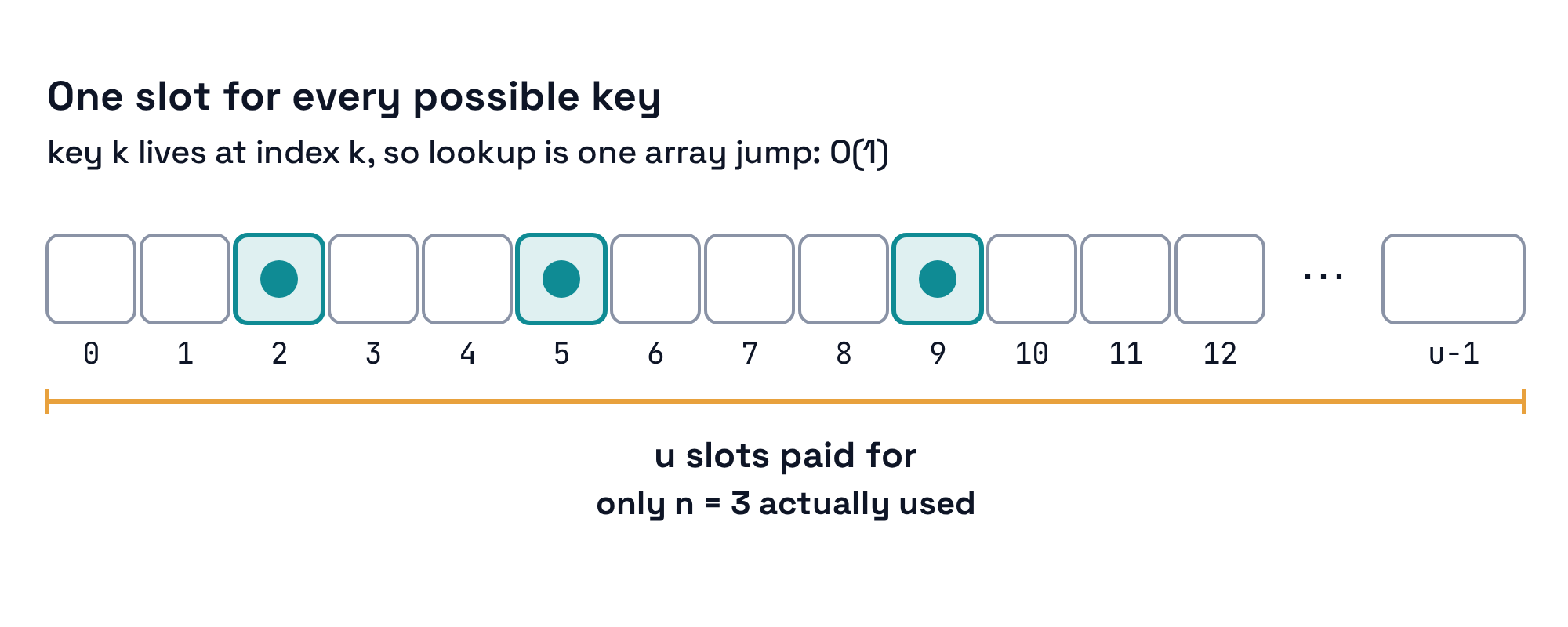
insert, delete, and find are each one array jump: worst case \(O(1)\). No comparisons anywhere.

The catch: space

The array needs one slot for every key that could ever occur, not just the ones present. Call that universe size \(u\).
Space is \(\Theta(u)\), and \(u\) is usually astronomical. Keys that are 10-letter names: \(u = 26^{10} \approx 141\) trillion slots, around 17.6 terabytes, to store one class roster.
The dream dies on the gap between \(n\) what we store and \(u\) what we might store.

What we want: direct access speed, but with a table of size \(m \approx n\). So the keys must be squashed into \(m\) slots.

Hashing: squash the universe

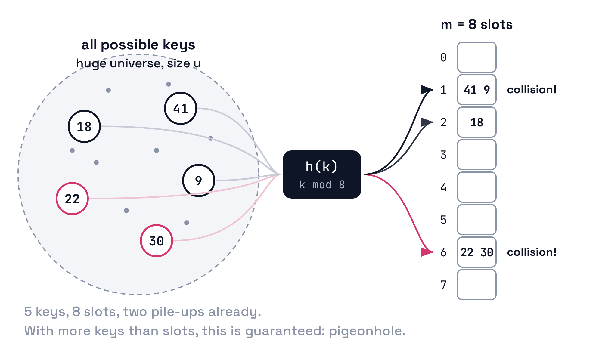
A hash function \(h\) maps every possible key to a slot number in \(\{0, 1, \ldots, m-1\}\). Store key \(k\) at slot \(h(k)\). Simplest example: \(h(k) = k \bmod m\).

Collisions are mandatory

The universe has \(u\) possible keys and the table has \(m \ll u\) slots, so some two keys must share a slot. That is the pigeonhole principle: \(u\) pigeons, \(m\) holes, \(u > m\).
No cleverness in choosing \(h\) can prevent this. For any \(h\), some slot has at least \(u/m\) possible keys mapped to it.
So collisions are not a bug to eliminate. They are a fact to manage.

Two questions decide everything: where do colliding keys go, and how long do the pile-ups get?

Chaining

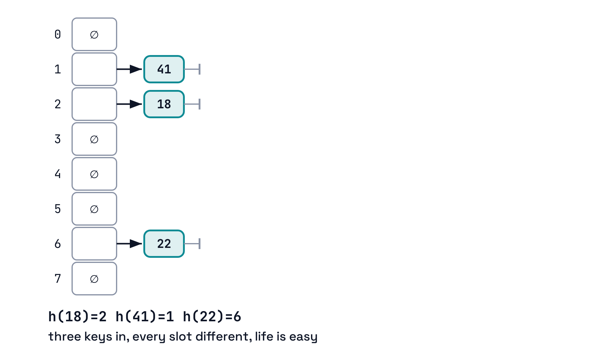
Each slot holds a list

Insert keys \(18, 41, 22\), then \(30\), then \(9, 14\) into \(m = 8\) slots with \(h(k) = k \bmod 8\):

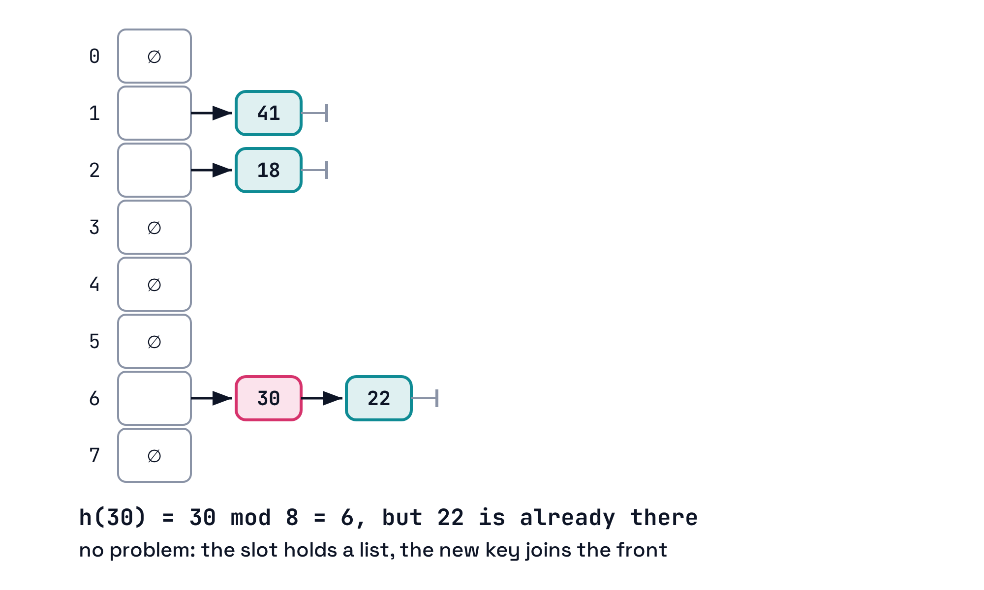
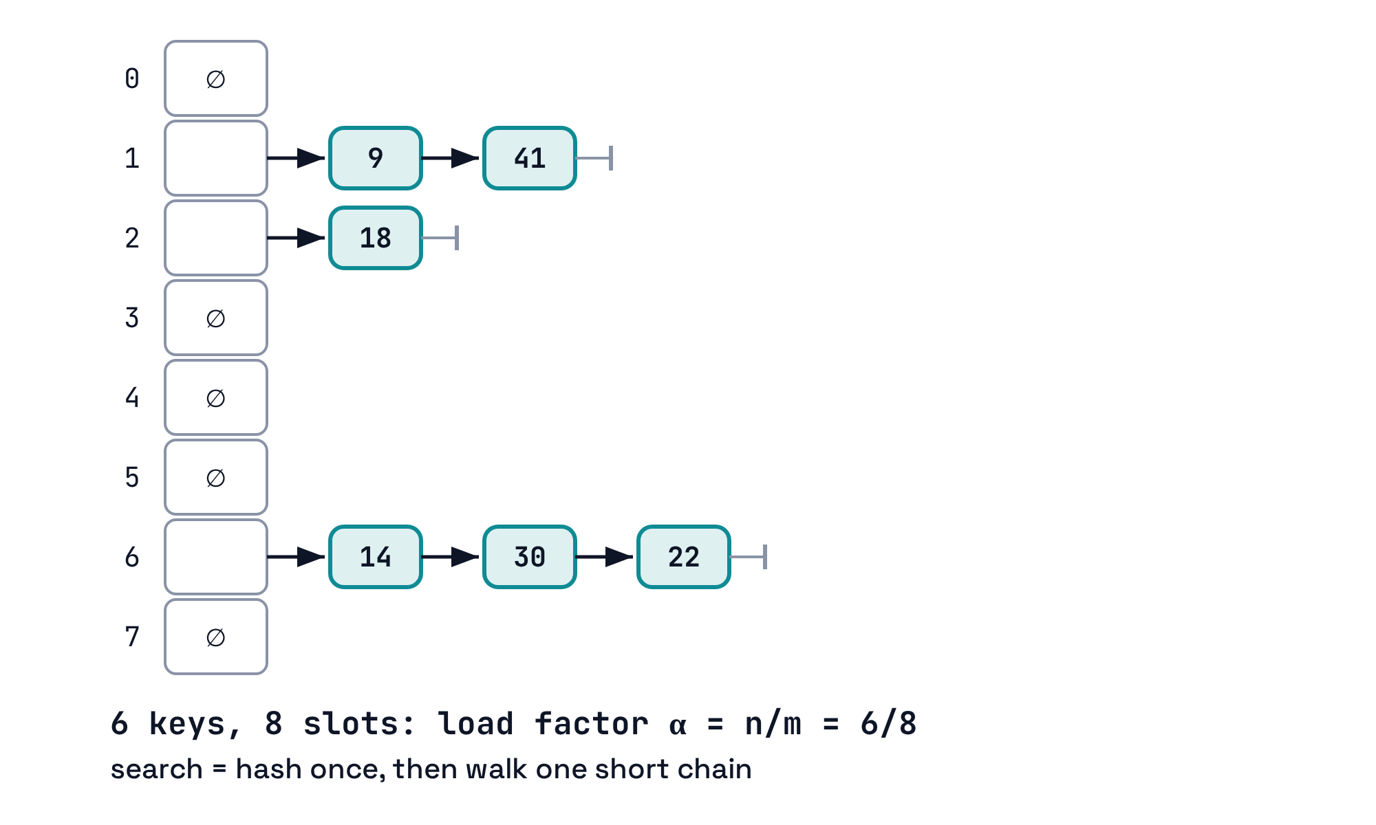
Operations under chaining

Every operation is “hash once, then deal with one chain”:

insert(x): compute \(h(k)\), prepend to that slot’s list. \(O(1)\): hashing is constant, prepending to a linked list is constant
find(k): compute \(h(k)\), walk that chain comparing keys until found or the chain ends. cost = length of that one chain
delete(k): same walk, then unlink. cost = length of that one chain

So the entire performance question collapses to one number: how long are the chains? In the best spread, length \(\approx 1\). In the worst pile-up, one chain of length \(n\) and the table is just a linked list wearing a costume.

Activity: hashing by hand

Your turn, in pairs

Take one worksheet per pair.

Side 1: build a table with \(m = 8\) slots and \(h(k) = k \bmod 8\). Insert the nine keys in the order given, drawing every chain. Then read off the longest chain, the load factor, and the cost of two searches.

Side 2: now be the villain. Choose keys that force all of them into one chain. Then fix the table so your own attack fails.

10 minutes. Worksheets come in at the end; one per pair, both names on it.

Debrief: side 1

Keys \(25, 14, 3, 22, 41, 16, 30, 7, 19\) with \(h(k) = k \bmod 8\):

Slot	Chain (newest first)
0	\(16\)
1	\(41 \to 25\)
3	\(19 \to 3\)
6	\(30 \to 22 \to 14\)
7	\(7\)

Longest chain: \(3\). Load factor: \(\alpha = 9/8\). find(30) compares once; find(14) walks all of slot 6’s chain: three comparisons. Slots 2, 4, 5 sit empty while slot 6 does triple duty. Averages hide unevenness.

Debrief: side 2

The villain’s move: pick keys that are all multiples of 8, say \(8, 16, 24, 32, 40\). Every one hashes to slot 0. One chain holds everything, and find is back to \(\Theta(n)\).
The trap is that \(k \bmod 8\) only looks at the low bits of \(k\), and real-world keys love patterns: addresses aligned to 8, prices ending in 0, IDs issued in blocks.
The classic patch: make \(m\) prime. With \(m = 7\), those same keys spread to slots \(1, 2, 3, 4, 5\). A prime shares factors with almost nothing, so arithmetic patterns stop lining up with the table size.

A patch, not a cure: for any fixed \(h\), some set of keys still piles up (pigeonhole again). Hold that thought for the fine print.

How long are the chains?

Probability in one minute

The chains depend on where keys happen to land, so the analysis needs one tool from HW0: expectation.

The expected value of a random quantity is its average over the randomness, weighted by probability. A fair die: \(\frac{1}{6}(1) + \frac{1}{6}(2) + \cdots + \frac{1}{6}(6) = 3.5\).
An indicator trick: if an event happens with probability \(p\), then “1 if it happens, 0 if not” has expected value exactly \(p\).
Expectations add. The expected value of a sum is the sum of the expected values, always, even when the pieces influence each other. This is the single most useful fact in the analysis of randomness.

The cast of characters

Three symbols run the whole analysis, in plain words:

Symbol	Meaning
\(n\)	how many keys are stored in the table
\(m\)	how many slots the table has
\(\alpha = n/m\)	the load factor: the average number of keys per slot

\(\alpha\) is the table’s crowding gauge. \(\alpha = 9/8\) from the activity: nine coats, eight hooks. Read \(n\) and \(m\) off the table; compute \(\alpha\). Same three every time.

Expected search cost, line by line

Assume simple uniform hashing: each key is equally likely to land in each of the \(m\) slots, independently of the others. Search for a key \(k\) that is not in the table:

Cost \(= 1 + (\text{length of chain at } h(k))\) one hash, then walk that whole chain to conclude “absent”
\(\text{length of chain at } h(k) = \sum_{\text{stored keys } x} \mathbf{1}[x \text{ landed there}]\) the chain is just a head-count of the stored keys that landed in that slot
\(E[\mathbf{1}[x \text{ landed there}]] = \frac{1}{m}\) each stored key had probability \(1/m\) of landing in the searched slot
\(E[\text{chain length}] = n \cdot \frac{1}{m} = \alpha\) expectations add: \(n\) keys, \(1/m\) each
\(E[\text{cost}] = 1 + \alpha = \Theta(1 + \alpha)\) a successful search is no worse: it stops partway down the same chain

The punchline

Expected search cost is \(\Theta(1 + \alpha)\). Keep the table sized so that \(m \approx n\), and \(\alpha\) stays below a constant, making every dictionary operation expected \(\Theta(1)\). The whole game of hashing is keeping \(\alpha\) small.

Three ways to charge for time

Today completes the course’s set of cost meanings. All three are averages of a sort, but over different things:

Kind	Averaged over	The promise	Seen with
Worst case	nothing	every single call is this fast	binary search
Amortized	a sequence of your calls	the sequence’s total is this fast, guaranteed	dynamic array append (Week 1)
Expected	the randomness	fast on average; any one call might be slow	hashing, today

The distinctions matter when things go wrong: an amortized bound cannot be defeated, but an expected bound can be, by bad luck or by an adversary. Hence the fine print, coming up.

Keeping the promise

Growing the table

\(\Theta(1 + \alpha)\) is only \(\Theta(1)\) while \(\alpha\) stays small, but \(n\) grows as keys arrive. The fix is one you have already seen:

When \(\alpha\) crosses a threshold (say \(\alpha > 1\)), allocate a table twice as big and re-insert everything. rehash into the new table: every key’s slot changes because \(m\) changed
One rebuild costs \(\Theta(n)\), but doubling means the next rebuild is \(n\) insertions away. Averaged over the sequence, each insert pays \(O(1)\) extra.
This is exactly the dynamic-array doubling argument from Week 1, reused unchanged. Rare big bills, amortized to pocket change.

So insert is amortized expected \(O(1)\): both meanings of “average,” working the same shift.

The fine print

The \(\Theta(1)\) promise has conditions. It stays honest only if you know them:

The worst case is still \(\Theta(n)\). Nothing prevents all \(n\) keys from sharing one chain; the analysis says it is unlikely, not impossible.
“Unlikely” assumed the keys spread out. \(k \bmod m\) is a heuristic: fine for messy keys, terrible for patterned ones, as side 2 of the worksheet proved. A fixed, published \(h\) can even be attacked on purpose.
The real cure is randomness in \(h\) itself. Choose the hash function at random from a well-designed family when the table is built, and the expected bound holds for every set of keys; no adversary can aim at a target they cannot see. The construction is called universal hashing: CLRS 11.3 for the curious.

Hashing in the wild

You have been using today’s data structure all along:

Every Python dict and set is a hash table. d[k], k in d, and d[k] = v are all expected \(O(1)\), which is why nobody thinks twice before using them inside a loop.
Python resolves collisions with a different plan (open addressing: colliding keys probe for a nearby empty slot) but the load-factor logic is the same, and the table doubles when \(\alpha\) gets large, just like today.
Strings hash fine: a string is just a large number in disguise (its bytes), and Python randomizes its string hash at startup, a real-world deployment of the fine print.

The scorecard

Where dictionaries stand after today, on \(n\) stored items:

Operation	Sorted array	Hash table (chaining)
`find(k)`	\(\Theta(\log n)\)	\(\Theta(1)\) expected
`insert(x)`	\(\Theta(n)\)	\(\Theta(1)\) amortized expected
`delete(k)`	\(\Theta(n)\)	\(\Theta(1)\) expected
`find_min()`	\(\Theta(1)\)	\(\Theta(n)\)
next-larger, range queries	\(\Theta(\log n)\)	\(\Theta(n)\)

Hashing bought speed by destroying order: \(h\) scatters keys on purpose, so the table knows nothing about which key is smallest. Getting find fast and the order operations fast at the same time needs a genuinely new structure. That story starts soon.

The one-slide version

Comparison-only search is stuck at \(\Omega(\log n)\), so hashing computes an address instead: squash the universe of keys into \(m \approx n\) slots with a hash function, and let each slot hold a chain. Collisions are guaranteed (pigeonhole), but with a good spread the chains average \(\alpha = n/m\) long, making every operation expected \(\Theta(1 + \alpha)\). Keep \(\alpha\) small by table doubling, amortized exactly like Week 1’s dynamic arrays. The promise is expected, not guaranteed: that is the price of the speed.

What’s next

Week 4 at a glance

Dr. Cordova is back Monday, September 14.

Supplemental reading (highly recommended): CLRS Chapter 11.

Upcoming deliverables:

HW1 due tonight at 9:59 PM.
HW2 is out today, due Monday, September 21 at 9:59 PM.

References

Sources

Cormen, T. H., Leiserson, C. E., Rivest, R. L., and Stein, C. Introduction to Algorithms, 4th edition, MIT Press. Chapter 11.
Carter, J. L. and Wegman, M. N. (1979). Universal classes of hash functions. Journal of Computer and System Sciences, 18(2), 143-154.