Linear Sorting

Lecture W4M1: Counting Sort, Radix Sort, and Sorting Without Comparing

Lucas P. Cordova, Ph.D.

lpcordova@willamette.edu

Willamette University

September 14, 2026

Before we begin: announcements

Three things worth knowing

I am back. Jet-lagged af, but back. Thank you to Sam for running Wednesday’s class on hashing.
HW2 is due Monday, September 21 at 9:59 PM. After today, every problem on it is fair game: the hashing problems from last week, and the sorting problems from today.
Wednesday we start binary trees, the structure that finally gets find fast and keeps the keys in order.

Learning objectives

What you will leave with

Explain what an amortized bound promises, what it does not, and how it differs from an expected bound.
Prove that any sort that only compares keys needs \(\Omega(n \log n)\) comparisons.
Trace counting sort on a small input and say why it is stable.
Trace radix sort, choosing the number of digits from \(n\) and the key range \(u\).
Choose the right sort for a workload from the size of the keys, and defend the choice with a cost.

Today’s goal

Last Wednesday we beat the \(\log n\) speed limit on find by computing where to look instead of comparing. Today we play the same trick on sorting, and beat \(n \log n\).

Last Wednesday, in review

Hashing in four bullets

The dictionary problem (insert, delete, find) has a speed limit if you only compare keys: \(\Omega(\log n)\) per find. Binary search is already optimal.
The way out: treat a key as a number, compute a slot \(h(k)\) from it, and go straight there. Squashing a huge universe of keys into \(m\) slots forces collisions (pigeonhole), so each slot holds a chain.
The cost is one hash plus one chain walk. With \(n\) keys in \(m\) slots, the expected chain length is the load factor \(\alpha = n/m\), so find is expected \(\Theta(1 + \alpha)\).
Keep \(\alpha\) small by doubling the table when it fills, and every operation is expected \(\Theta(1)\).

The picture to keep

Nine keys, eight slots, \(h(k) = k \bmod 8\):

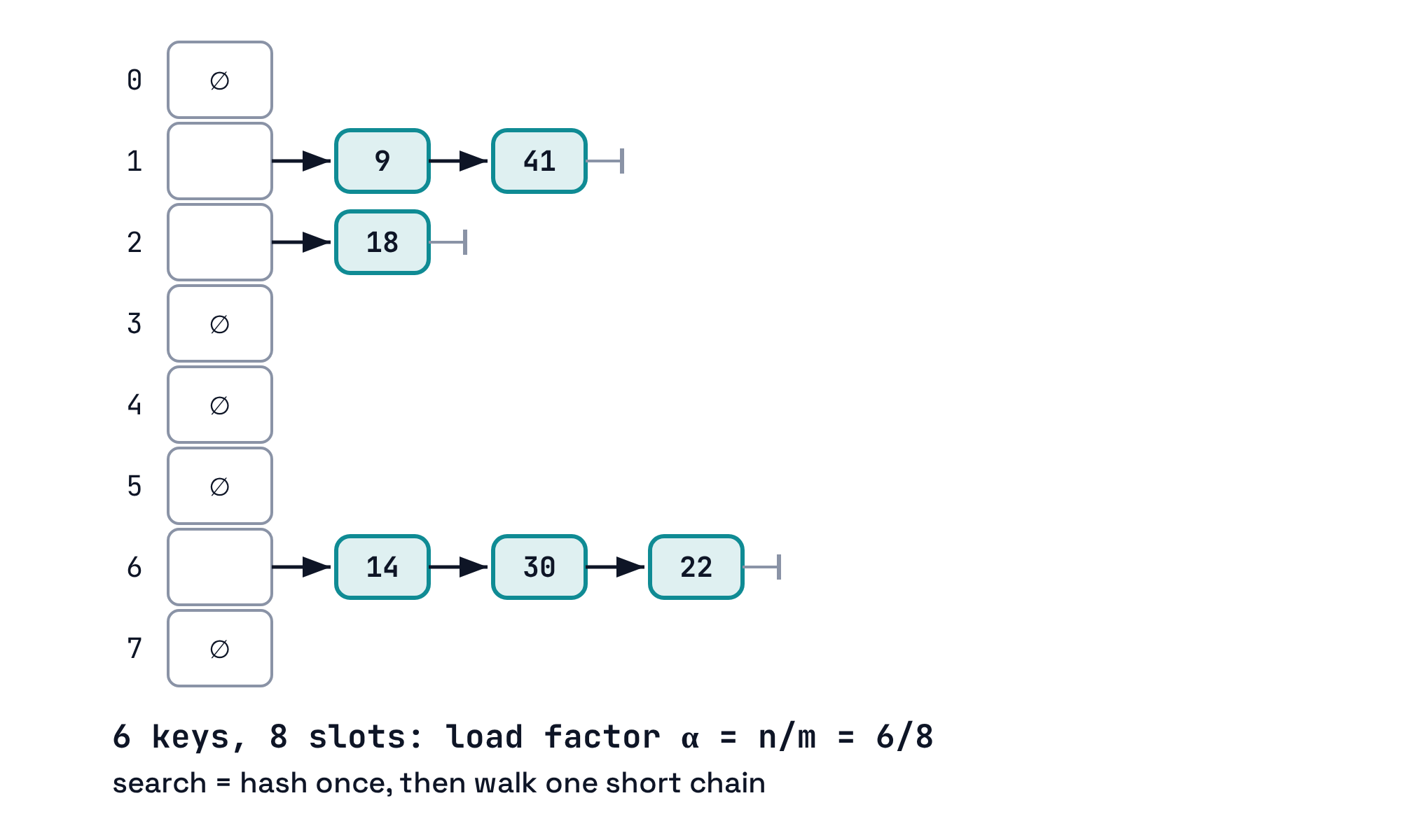
Same three numbers every time: \(n\) stored keys, \(m\) slots, \(\alpha = n/m\) keys per slot on average. Read \(n\) and \(m\) off the table and \(\alpha\) tells you the expected cost.

The word that deserves a second pass

Two different words for “average” showed up last week, and they are not interchangeable:

Expected \(\Theta(1)\): average over the randomness. Any single find might be slow if the keys happened to pile up.
Amortized \(\Theta(1)\): average over a sequence of your own calls. No randomness anywhere; a guarantee about the total.
Hash-table insert uses both at once: expected for the chain, amortized for the occasional table doubling.

Amortized is the one that trips people up, so let us rebuild it from scratch with numbers.

Amortization, rebuilt with numbers

The setting

Amortized analysis exists for one specific situation:

Most operations are cheap.
Once in a while, one operation is expensive.
The expensive ones are rare in a provable way: doing an expensive one buys you a long stretch of cheap ones.

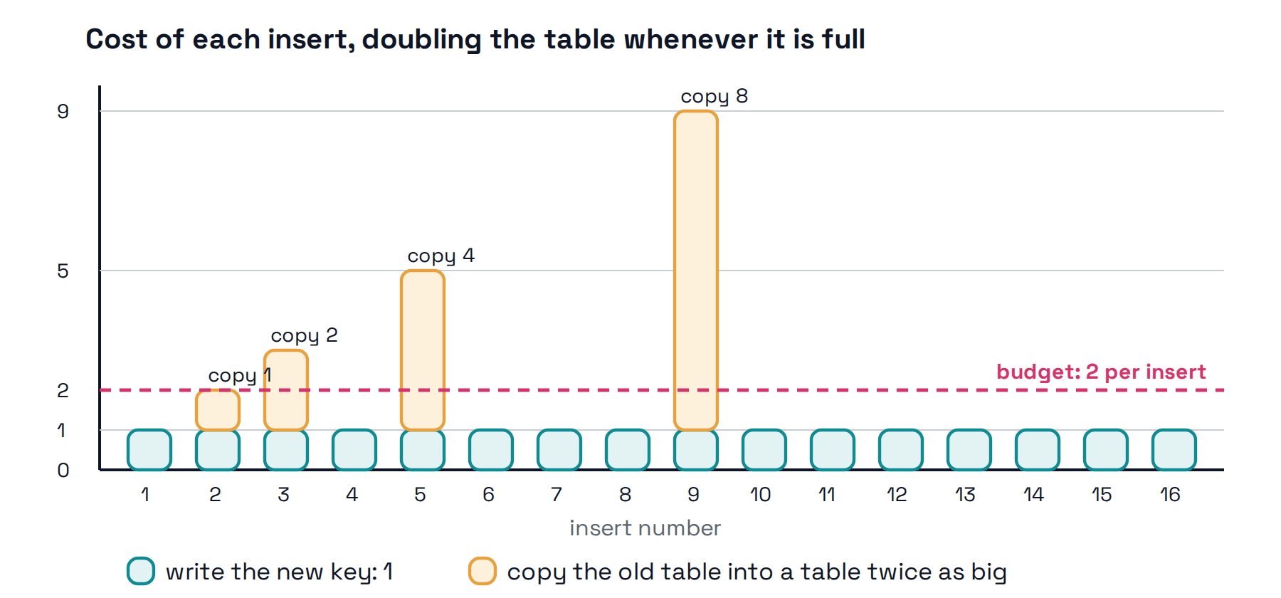
Doubling a table when it fills is the textbook example. Watch sixteen inserts into a table that starts with room for one key.

Sixteen inserts, one ledger 💷

Check, please! 🧾

Do the arithmetic, line by line:

Writing each new key: \(16 \times 1 = 16\) every insert pays this
Copies, when the table fills: \(1 + 2 + 4 + 8 = 15\) each copy is twice the last, and the last copies half the keys
Total: \(16 + 15 = 31 < 2 \times 16\) less than two units of work per insert
In general, copies cost \(1 + 2 + 4 + \cdots + n/2 < n\) a doubling series adds up to less than its next term
Total for \(n\) inserts \(< n + n = 2n\), so each insert is amortized \(O(1)\) the total is what we promise; divide by \(n\) for the per-operation figure

Numeric check

Suppose \(n = 1{,}000{,}000\) inserts. The copies happen at sizes \(1, 2, 4, \ldots, 524{,}288\): twenty of them, totaling \(1{,}048{,}575\). Together with the million writes, that is about \(2.05\) million units of work for a million inserts.

The single biggest insert cost half a million by itself. And the average is still about \(2\). That is the whole idea: rare and expensive averages out against frequent and cheap. ✔︎

What amortized promises (and doesn’t)

An operation runs in amortized time \(T(n)\) if any sequence of \(k\) of these operations costs at most \(k \cdot T(n)\) in total.

It is a promise about totals, for every possible sequence. No luck involved, and no adversary can break it.
It is not a promise about any single call. One append can still pause to copy everything.
It is the right cost to quote when you care about the whole run of a program, which is almost always.

Quick check: true or false? 🤔

Appending to a Python list is amortized \(O(1)\), so every single append takes \(O(1)\) time. False. The occasional resize is \(\Theta(n)\). The guarantee is about the total.
If a program does \(1000\) appends, the total work is \(O(1000)\). True. That is exactly what amortized \(O(1)\) means.
Hash-table find is amortized \(O(1)\). False. It is expected \(O(1)\). A bad spread of keys makes every find slow, and averaging over your calls does not rescue you.

Quick check, continued 🤔

A table that doubles when full and halves when exactly half full stays amortized \(O(1)\) per operation. False. Alternate one insert and one delete at the boundary and every operation resizes: \(\Theta(n)\) each. Week 1’s fix: shrink only at one quarter full, so there is a gap between the two triggers.
Hash-table insert is “amortized expected” \(O(1)\). True. Expected because of the chain walk; amortized because of the occasional doubling. Two different averages, each covering a different part of the cost.

Three ways to charge for time 🧾

Kind	Averaged over	The promise	Seen with
Worst case	nothing	every single call is this fast	binary search, merge sort
Amortized	a sequence of your calls	the sequence’s total, guaranteed	dynamic array append, table doubling
Expected	the randomness	fast on average; any one call might be slow	hashing

When an exam asks “what is the running time,” it will say which kind it wants. When it does not, worst case is the default.

The one-line version

Amortized means “the total over any sequence is bounded, guaranteed.” Expected means “the average over the randomness is bounded, but you might get unlucky.” Both can be \(O(1)\); only one of them is a promise about your particular run.

Today’s question

Faster than merge sort?

Last week’s scorecard, plus one column we have not filled in:

Structure	`build`	`find(k)`	`insert`	`find_min`
Unsorted array	\(n\)	\(n\)	\(n\)	\(n\)
Sorted array	\(n \log n\)	\(\log n\)	\(n\)	\(1\)
Hash table	\(n\) (expected)	\(1\) (expected)	\(1\) (amortized expected)	\(n\)

build for a sorted array is sorting, and merge sort’s \(\Theta(n \log n)\) is the best we have. Is \(n \log n\) a law of nature, or just a limit on comparing?

Comparison sorting has a speed limit 🚄

Suppose a sorting algorithm learns about the keys only by comparing pairs. Each comparison has at most \(3\) outcomes.

After \(t\) comparisons, the algorithm can be in at most \(3^t\) distinct states. same counting as last week: each answer splits the possibilities three ways
Sorting \(n\) distinct keys has \(n!\) possible correct answers: one for each ordering the input could have been in. a different input order needs a different rearrangement, so the algorithm must be able to end in \(n!\) ways
So \(3^t \geq n!\), which gives \(t \geq \log_3(n!)\). fewer states than answers means two inputs get the same, wrong, output

From \(\log(n!)\) to \(n \log n\)

\(n! = n \cdot (n-1) \cdots 2 \cdot 1\) has \(n\) factors, and the largest \(n/2\) of them are each at least \(n/2\). drop the small factors; the product only gets smaller
So \(n! \geq (n/2)^{n/2}\). \(n/2\) factors, each at least \(n/2\)
Take logs: \(\log(n!) \geq \frac{n}{2} \log \frac{n}{2} = \Omega(n \log n)\). logs turn the power into a product
Therefore \(t = \Omega(n \log n)\) comparisons, for any comparison-based sort, on some input. the lower bound is about the problem, not about one algorithm

Check with \(n = 8\): \(8! = 40{,}320\) and \((8/2)^{8/2} = 256\). Comfortably true.

Merge sort is optimal, then

Among algorithms that only compare keys, merge sort’s \(\Theta(n \log n)\) cannot be beaten. Any faster sort must be doing something other than comparing: the same escape hatch that made hashing fast.

Sorting by computing, not comparing

The direct-access dream, again

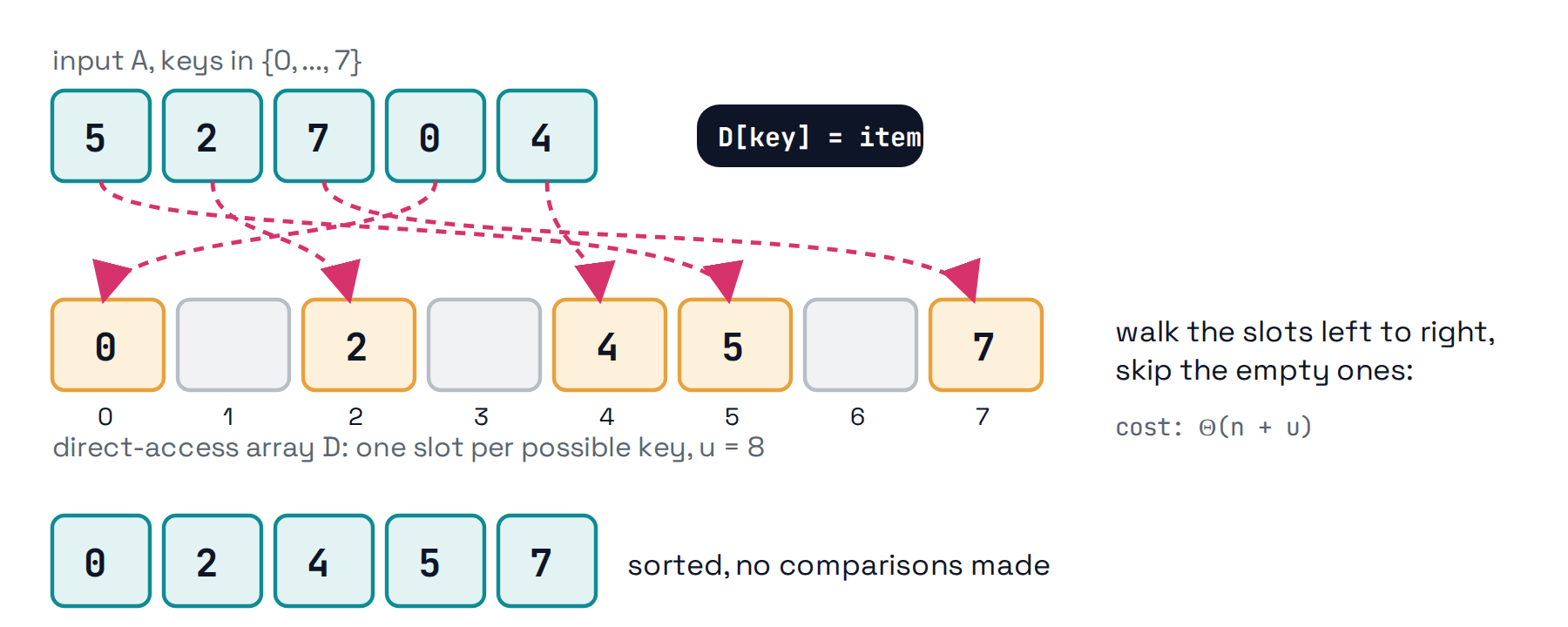
Suppose the keys are distinct integers in \(\{0, 1, \ldots, u - 1\}\). Put each item in slot key of an array with \(u\) slots, then read the slots in order:

Direct-access sort, priced

Find the largest key to size the array: \(O(n)\).
Place each item at D[x.key]: \(n\) writes, \(O(1)\) each.
Walk the \(u\) slots and read out the non-empty ones: \(O(u)\).
Total: \(\Theta(n + u)\). When \(u = O(n)\), that is \(\Theta(n)\). Linear time, and not one comparison.

Two catches, though. Keys had to be distinct (two items cannot share a slot), and \(u\) had to be small (a key range of \(n^2\) would cost \(\Theta(n^2)\) just to walk). Counting sort fixes the first; radix sort fixes the second.

Catch one: repeated keys

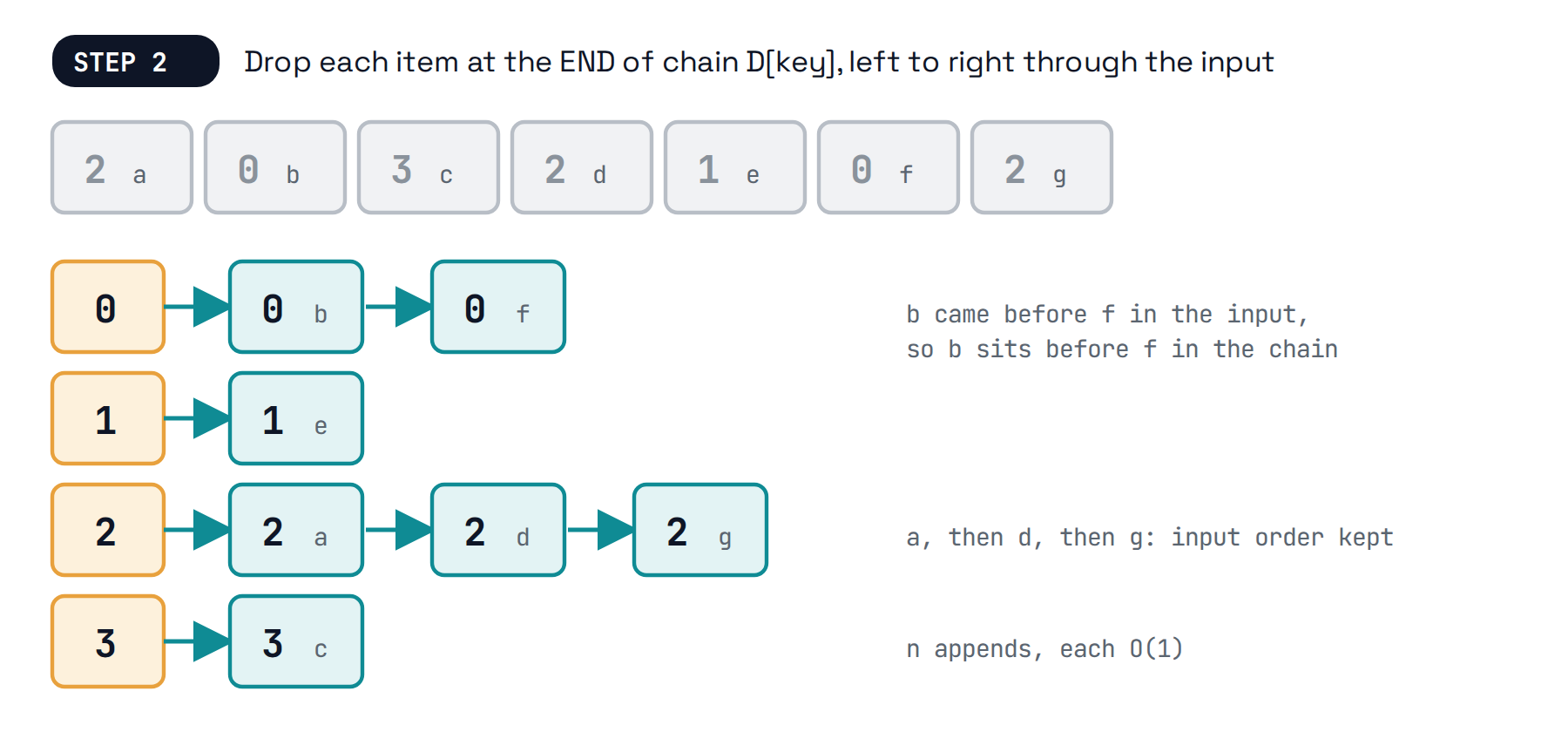
Store a chain at each slot, exactly like hashing, but with a rule about order:

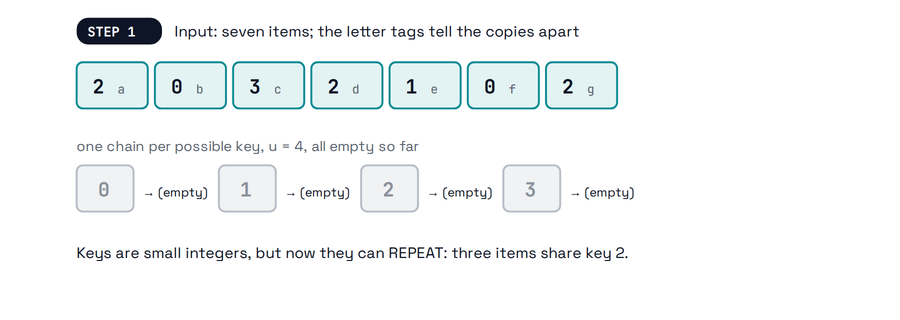
Counting sort

def counting_sort(A: list) -> None:
    "Sort A by x.key, assuming keys are integers in 0..u-1"
    u = 1 + max(x.key for x in A)      # O(n)   find the key range
    D = [[] for _ in range(u)]         # O(u)   one chain per possible key
    for x in A:                        # O(n)   append to the END of chain x.key
        D[x.key].append(x)
    i = 0
    for chain in D:                    # O(n+u) read chains back in slot order
        for x in chain:
            A[i] = x
            i += 1

Cost: \(\Theta(n + u)\), same as before, and now repeated keys are fine. Appending to the end of each chain is what makes it stable.

Stability, in plain words

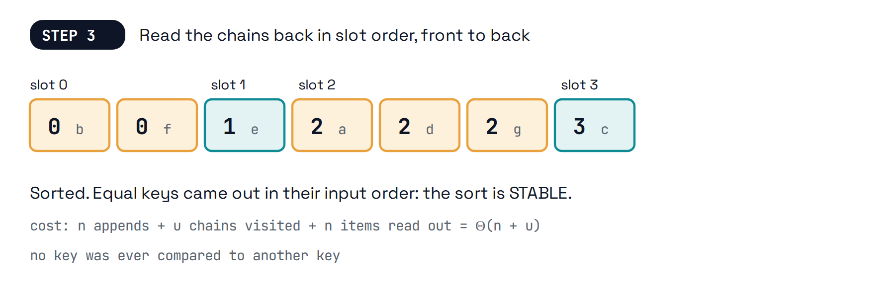
A sort is stable if items with equal keys come out in the same relative order they went in.

In the graphic, \(b\) came before \(f\) in the input, and \(b\) came out before \(f\). Same for \(a, d, g\).
Why anyone cares: sort a spreadsheet by last name, then by state. If the second sort is stable, each state’s block is still alphabetical. If not, the first sort was wasted.
Merge sort is stable (take from the left half on ties). Counting sort is stable. Most fast in-place sorts are not. Radix sort is the spreadsheet trick, run on the digits of a number.

The bookkeeping version

CLRS writes counting sort without chains. Instead of building lists, it works out where each key’s block will sit in the sorted output, then drops every item straight into its final position.

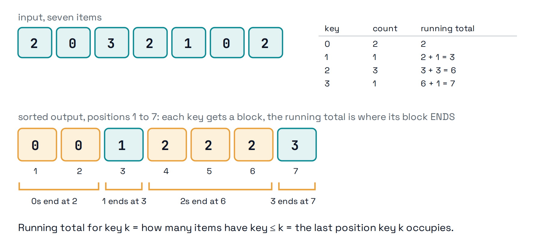
Reading the running totals

Count each key: \(C = [2, 1, 3, 1]\). two 0s, one 1, three 2s, one 3
In the sorted output, the 0s must fill positions \(1\) to \(2\), then the 1 takes position \(3\), then the 2s fill \(4\) to \(6\), then the 3 takes \(7\). sorted means every 0 before every 1 before every 2 before every 3
The running total \(2, 2{+}1, 3{+}3, 6{+}1 = [2, 3, 6, 7]\) is exactly the last position of each block. running total for key \(k\) = how many items have key \(\le k\)
So \(C[k]\) now answers “where does key \(k\)’s block end?” That is the only table the placement step needs.

Placing from the back

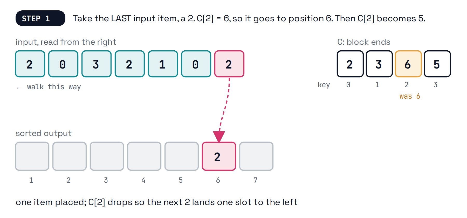
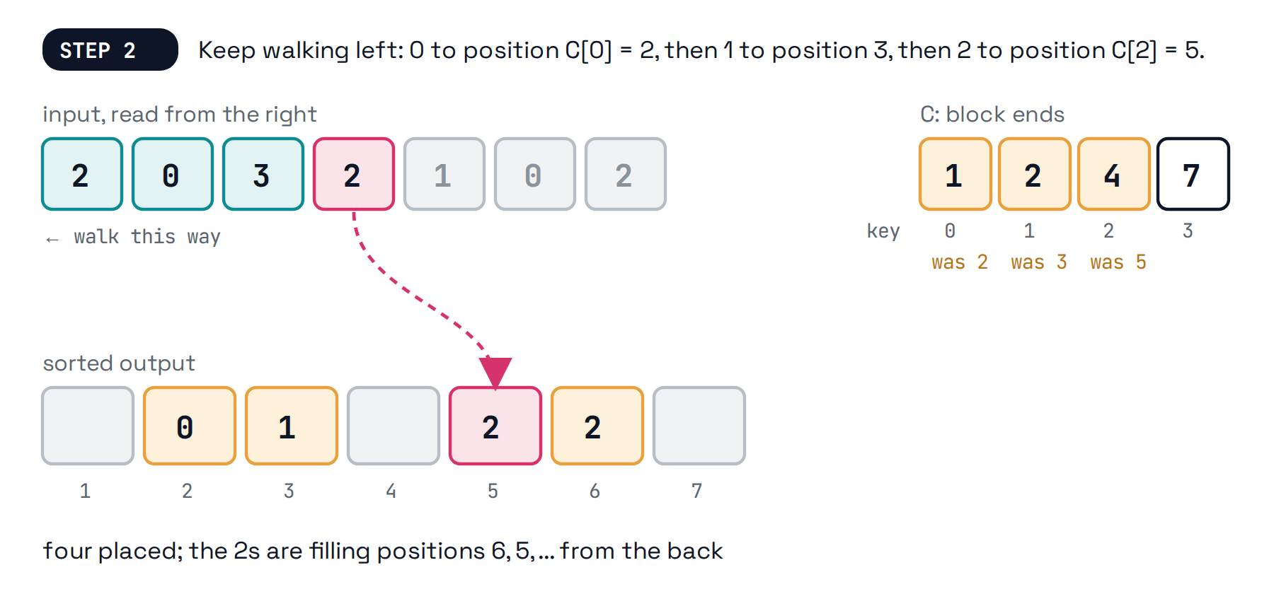
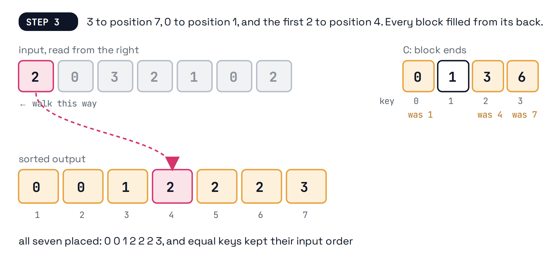
Walk the input backwards. Each item goes to position \(C[\text{key}]\), and then \(C[\text{key}]\) drops by one:

Why that is stable

\(C[2]\) started at \(6\), the end of the 2s’ block, so the first 2 we met (the last one in the input) took the last 2-slot. decrementing walks the pointer toward the front of the block
The next 2 we met took slot \(5\), and the first 2 of the input took slot \(4\). backwards through the input, backwards through the block
Two reversals cancel: the input order of equal keys is the output order. Stable, with no chains anywhere.

Two versions, one sort

Chains or running totals, counting sort costs \(\Theta(n + u)\) and is stable either way. The running-total version just replaces “append to a list” with “know in advance where the list would have ended.” Either version is fine on an exam; say which one you are using.

Catch two: big keys

When \(u\) is too big

Counting sort is \(\Theta(n + u)\). That is only linear while \(u = O(n)\).

Sorting \(n = 1000\) keys that are 9-digit ID numbers: \(u = 10^9\). Counting sort would walk a billion slots to sort a thousand items. Merge sort would take about \(10{,}000\) steps.
The idea: do not treat the key as one number. Treat it as a few digits, each digit small enough for counting sort.
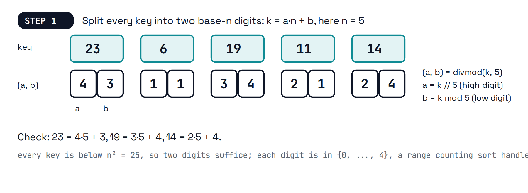
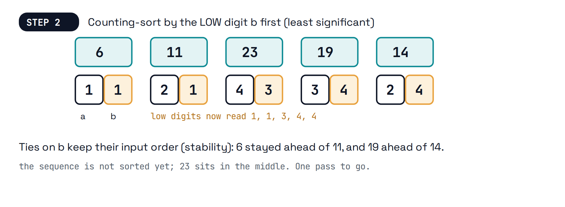
Which digits? Not decimal ones. Divide the key by \(n\): the quotient is the high digit and the remainder is the low digit. With \(n = 5\), the key \(23 = 4 \cdot 5 + 3\) becomes the pair \((4, 3)\).

Two digits, base \(n\)

In symbols, with \(a\) for the quotient and \(b\) for the remainder:

\(k = a \cdot n + b\), where \(a = \lfloor k / n \rfloor\) and \(b = k \bmod n\). Python: a, b = divmod(k, n)
Both digits are in \(\{0, \ldots, n-1\}\): \(b\) because it is a remainder mod \(n\), and \(a\) because \(k < n^2\) means \(k / n < n\). exactly the key range counting sort likes
Check: \(n = 5\), \(k = 19\). \(19 = 3 \cdot 5 + 4\), so \((a, b) = (3, 4)\), and both digits are below \(5\). and \(19 < 25 = n^2\), as required

Then sort by digits, one at a time. The order of the passes is the whole trick.

Radix sort, on five keys

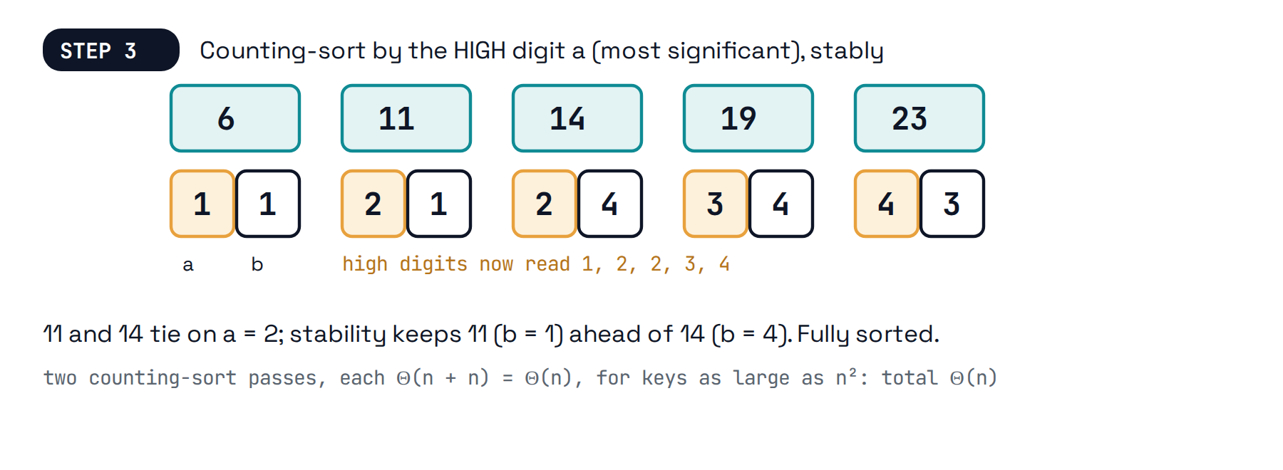
\(n = 5\) keys, \(23, 6, 19, 11, 14\), all below \(n^2 = 25\):

Why least significant digit first?

The passes go from the least significant digit to the most significant, and every pass must be stable:

After the last pass (the high digit), keys with different high digits are in the right order. the high digit decides
Keys with the same high digit were left in the order the previous pass put them in, which was sorted by the low digit. that is what stable means
So ties on the high digit are broken correctly by the low digit, for free. the earlier pass did the work; stability preserved it

Try it the other way round (high digit first) and the second pass scrambles the first. Sort a spreadsheet by state and then by last name, and the states are gone.

Radix sort, priced

The cast of characters, in plain words:

Symbol	Meaning
\(n\)	how many keys
\(u\)	how big the keys can get: every key is below \(u\)
\(c\)	how many base-\(n\) digits it takes to write a key

Each pass is one counting sort on digits in \(\{0, \ldots, n-1\}\): \(\Theta(n + n) = \Theta(n)\). \(n\) items, \(n\) possible digit values
One pass per digit, so \(c\) passes: total \(\Theta(c \cdot n)\). the whole cost rides on how many digits a key needs

How many digits is \(c\)?

With \(c\) digits in base \(n\), the biggest number you can write is \(n^c - 1\). every digit at its maximum, \(n - 1\); compare: three decimal digits reach \(999 = 10^3 - 1\)
So \(c\) digits are enough for every key exactly when \(n^c \geq u\). the largest key must fit
Take \(\log_n\) of both sides: \(c \geq \log_n u\), so the smallest that works is \(c = \lceil \log_n u \rceil\). logs undo powers
Substitute into \(\Theta(c \cdot n)\): radix sort costs \(\Theta(n \log_n u)\). \(c\) was the only unknown
If \(u \leq n^c\) for a constant \(c\), that is \(c\) passes of \(\Theta(n)\) each: \(\Theta(n)\). Linear. \(u = n^2\) means \(2\) passes; \(u = n^3\) means \(3\)

Numeric check

\(n = 1000\) keys below \(10^9\): \(c = \lceil \log_{1000} 10^9 \rceil = 3\) passes. About \(3 \times 2000 = 6000\) steps. Merge sort: about \(1000 \times 10 = 10{,}000\) comparisons. Radix wins, and the gap widens with \(n\).
Same keys in base 10 instead of base \(n\): \(9\) passes. Base \(n\) is the right base because it makes each pass as cheap as it can be while using as few passes as possible.
\(n = 1000\) keys below \(2^{64}\): \(c = \lceil 64 / \log_2 1000 \rceil = \lceil 6.4 \rceil = 7\) passes. Still linear, still constant \(c\).
\(n\) keys with no bound on \(u\): \(c\) is not a constant, and radix sort’s \(\Theta(n \log_n u)\) can lose to merge sort. Then compare.

Where the keys came from

A string of \(d\) characters over an alphabet of size \(s\) is a \(d\)-digit number in base \(s\): radix sort by character, last character first, \(d\) stable passes.
A tuple \((x, y)\) is a two-digit key. Sort by \(y\), then stably by \(x\).
A fraction \(p/q\) with all \(q\) equal: sort by \(p\). A fraction \(p / n^2\) between \(0\) and \(100\): \(p < 100 n^2\), so radix sort with three base-\(n\) passes.
A key that is a year: \(u\) is a few thousand at most. Counting sort, one pass.

The question to ask every time: how big can the key get, compared with \(n\)? The answer picks the sort.

Activity: sorting without comparing

Your turn, in pairs

Take one worksheet per pair.

Side 1: counting-sort eight tagged items by hand, chains and all, then read the sorted order and check stability.

Side 2: radix-sort seven 3-digit numbers, one pass per digit, then answer three “which sort?” questions from the size of the keys.

10 minutes. Worksheets come in at the end; one per pair, both names on it.

Debrief: side 1

Items \(3_A, 1_B, 4_C, 1_D, 0_E, 3_F, 1_G, 2_H\) with keys in \(\{0, \ldots, 4\}\):

Slot	Chain (front to back)
0	\(0_E\)
1	\(1_B \to 1_D \to 1_G\)
2	\(2_H\)
3	\(3_A \to 3_F\)
4	\(4_C\)

Output: \(0_E, 1_B, 1_D, 1_G, 2_H, 3_A, 3_F, 4_C\). The three 1s and the two 3s are in input order: stable. Cost \(\Theta(n + u) = \Theta(8 + 5)\).

Debrief: side 2

Keys \(512, 348, 152, 890, 341, 705, 148\), one stable pass per digit:

After the ones pass: \(890, 341, 512, 152, 705, 348, 148\)
After the tens pass: \(705, 512, 341, 348, 148, 152, 890\)
After the hundreds pass: \(148, 152, 341, 348, 512, 705, 890\). Sorted.

Watch \(348\) and \(148\): they tie on the tens pass (\(4\)), and stability kept \(348\) ahead because the ones pass had put it there. Then the hundreds pass separated them for good.

Debrief: which sort?

\(n\) exam scores, integers \(0\) to \(100\): \(u = 101\), so counting sort in \(\Theta(n + 101) = \Theta(n)\).
\(n = 2^{20}\) keys that are 64-bit integers: \(u = 2^{64} = n^{3.2}\), so radix sort with \(c = 4\) base-\(n\) passes: \(\Theta(n)\).
\(n\) recordings ranked by which one a judge prefers, one pair at a time: no numeric key at all, only comparisons. Merge sort, \(\Theta(n \log n)\), and the lower bound says nothing better exists.

Wrapping up

The sorting scorecard

Algorithm	Time	In place?	Stable?	When to reach for it
Insertion sort	\(O(n^2)\)	yes	yes	tiny or nearly sorted inputs
Merge sort	\(O(n \log n)\)	no	yes	any keys you can compare; optimal among comparison sorts
Counting sort	\(O(n + u)\)	no	yes	integer keys with \(u = O(n)\)
Radix sort	\(O(n \log_n u)\)	no	yes	integer keys with \(u = O(n^c)\), \(c\) constant

Python’s built-in sort is a comparison sort (a tuned merge sort called Timsort), because it has to work on anything. When your keys are small integers and \(n\) is large, you can beat it.

The fine print

Linear sorting needs integer keys (or things that become integers: characters, fixed-length strings, bounded fractions) in a known, bounded range. Arbitrary floats, or keys you can only compare, are out.
\(\Theta(n + u)\) hides a real cost when \(u \gg n\): counting sort on a thousand 9-digit numbers is a disaster. Check \(u\) against \(n\) before you commit.
Radix sort’s \(c\) must be a constant for the bound to be linear. If the keys grow without bound as \(n\) grows, be honest and write \(\Theta(n \log_n u)\).
These sorts are not in place: they need \(\Theta(n + u)\) extra space. Merge sort needs \(\Theta(n)\); insertion sort needs \(O(1)\).

The one-slide version

Any sort that only compares keys needs \(\Omega(n \log n)\) comparisons, because \(n!\) answers need \(\log(n!)\) three-way questions. To go faster, stop comparing and use the key as an address: counting sort drops items into chains indexed by key and reads them back in order, \(\Theta(n + u)\), stable. When keys are too big, radix sort splits each key into base-\(n\) digits and counting-sorts one digit at a time, least significant first, relying on stability to keep earlier passes intact: \(\Theta(n \log_n u)\), linear whenever \(u \leq n^c\). The question that picks the sort is always the same: how big are the keys, compared with \(n\)?

What’s next

Wednesday at a glance

Topics: Binary trees, part 1. A structure that keeps keys in order and makes find, insert, delete, and the order operations (find_min, next-larger, range queries) all logarithmic at once. The hash table’s missing column.

Supplemental reading (highly recommended): CLRS Chapter 8 for today; Chapter 12 for Wednesday.

Upcoming deliverables:

HW2 due Monday, September 21 at 9:59 PM on Canvas. Everything on it has now been covered.
Next Monday: HW3 goes out, and the semester project is assigned (teams of 3).

References

Sources

Cormen, T. H., Leiserson, C. E., Rivest, R. L., and Stein, C. Introduction to Algorithms, 4th edition, MIT Press. Chapter 8 (Sorting in Linear Time); Section 16.4 (Dynamic tables); Chapter 11 (Hash Tables).
CS 351 Syllabus: Canvas.