Binary Trees

Lecture W5M3: Binary Trees, Part 1

Lucas P. Cordova, Ph.D.

lpcordova@willamette.edu

Willamette University

September 21, 2026

Learning objectives

What you will leave with

Define a binary tree by its pointers, and its traversal order by one recursive rule.
Trace first, successor, insert-before/after, and delete on a small tree, each in \(O(h)\) time.
Explain how one tree shape implements both a Set (the BST property) and a Sequence (subtree sizes).
State why \(O(h)\) is only a promise once \(h = O(\log n)\), which is Wednesday’s job.

Today’s goal

Hash tables gave us \(O(1)\) find and nothing about order. Sorted arrays gave us order and \(O(n)\) insert. Today we build the structure that does both, and end with the one question it leaves open.

Today’s question

The gap we are closing today

Set interface	Sorted array	Hash table	Goal
`build(X)`	\(n \log n\)	\(n\) (e)	\(n \log n\)
`find(k)`	\(\log n\)	\(1\) (e)	\(\log n\)
`insert(x)`, `delete(k)`	\(n\)	\(1\) (a, e)	\(\log n\)
`find_min()`, `find_max()`	\(1\)	\(n\)	\(\log n\)
`find_prev(k)`, `find_next(k)`	\(\log n\)	\(n\)	\(\log n\)

Neither column gets every row. The goal column asks for every operation logarithmic, order operations included. (e) expected, (a) amortized

Binary trees

A pointer-based structure

Linked lists taught us that pointers give worst-case guarantees: no table doubling, no expected bounds. Their weakness is that a chain is long.
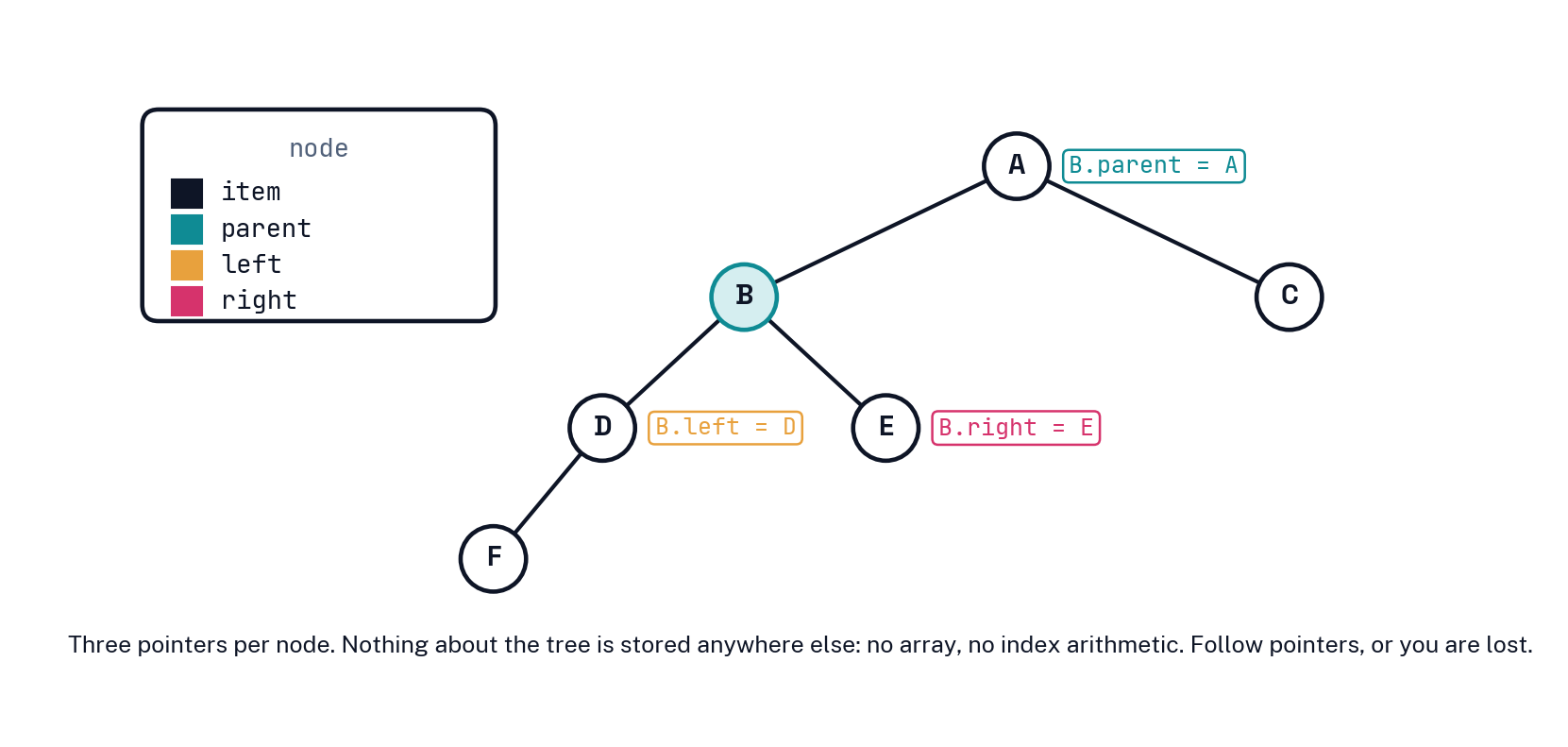
Fix: give each node three pointers instead of one.
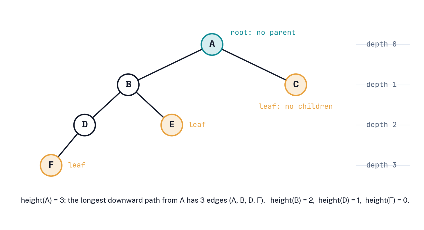
A node stores item, parent, left, right. Nothing else holds the tree together.
The root has no parent. A node with no children is a leaf.

The node, and a tree of six

Anatomy

Depth and height

The depth of a node is the number of edges on the path from the root to it. The height of a node is the length of the longest downward path from it to a leaf. The height \(h\) of the tree is the height of its root.

Every operation today runs in \(O(h)\): it walks one path down, or one path up.
The plan, in one sentence: design operations that cost \(O(h)\), then keep \(h = O(\log n)\).
Today is the first half. Wednesday is the second.

Traversal order

One rule gives the tree an order

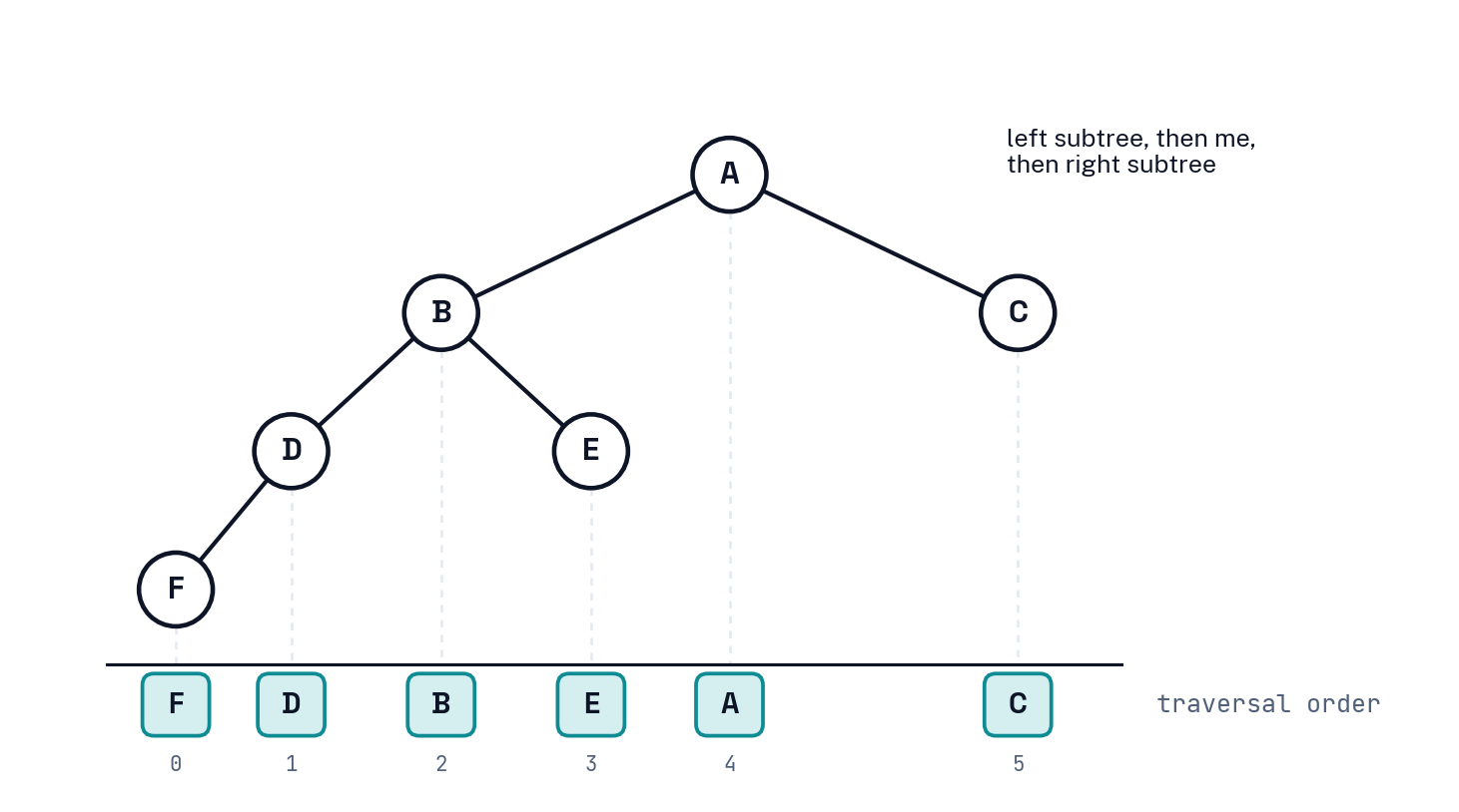
The traversal order of a binary tree is: everything in the left subtree, then the node itself, then everything in the right subtree, applied recursively.

Listing the order

list(X): list(X.left), then X, then list(X.right). Each node does \(O(1)\) work, so listing everything costs \(O(n)\).
For the tree above: \(F, D, B, E, A, C\).
Right now that order means nothing about the items. That is deliberate.
In a moment we will assign it a meaning: sorted by key (a Set), or position in a list (a Sequence). The algorithms below do not care which.

Quick check 🤔

Which node is first in traversal order? The leftmost node reachable by going left from the root: \(F\).
Which is last? Keep going right from the root: \(C\).
If a node has a right child, where is its successor? Somewhere in that right subtree. Which node in it?

First and last

subtree_first(X): if X.left exists, recurse on it; otherwise X is first.
subtree_last(X) is the mirror image: follow right pointers until you cannot.
Each step goes one level down, so the cost is \(O(h)\).
find_min and find_max for the Set will be exactly these two calls on the root.

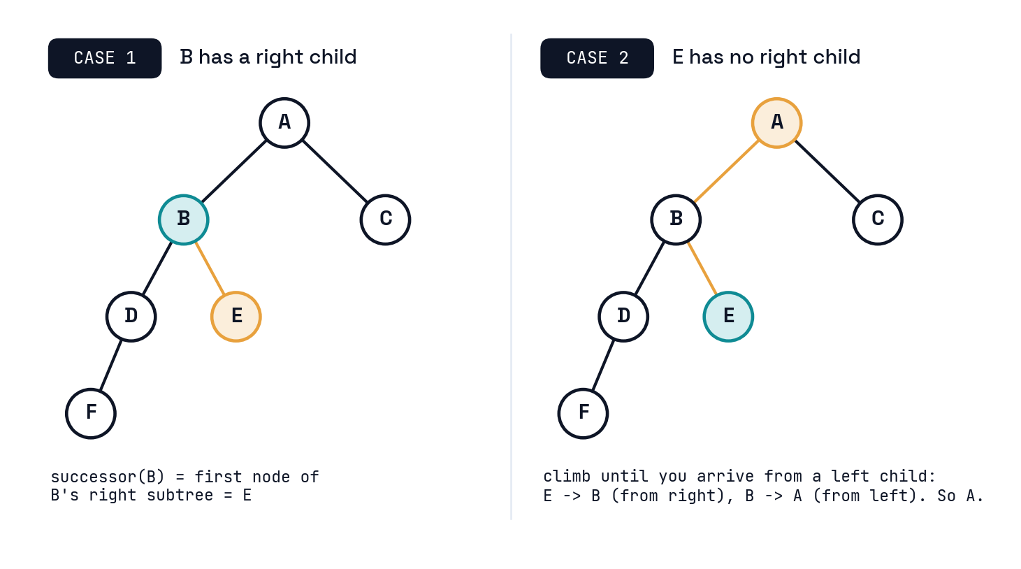
Successor: two cases

Successor, written out

successor(X): if X.right exists, return subtree_first(X.right).
Otherwise, walk up: climb parents until you arrive at a node from its left child. That node is the successor. If you reach the root without doing so, X was last.
Both cases follow a single path, down or up, so \(O(h)\).
predecessor is the mirror: subtree_last(X.left), or climb until you arrive from a right child.

Changing the tree

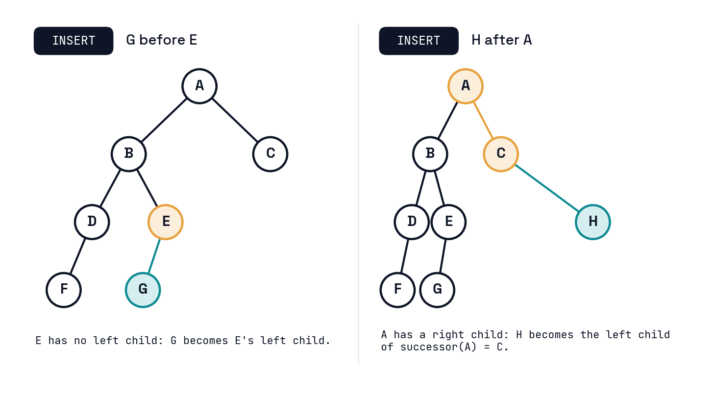
Insert: only ever add a leaf

insert_after(X, Y): if X.right is empty, make Y the right child of X.
Otherwise, make Y the left child of successor(X). Why is that slot guaranteed empty? If the successor had a left child, that child would come between them in traversal order.
insert_before is the mirror, using predecessor.
Cost: one successor call plus \(O(1)\) pointer surgery, so \(O(h)\).

Two inserts on the example

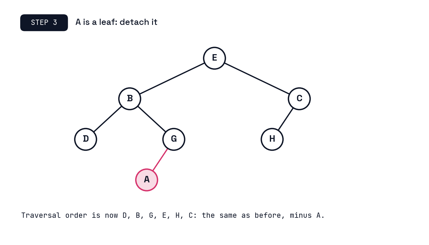
Delete: only ever remove a leaf

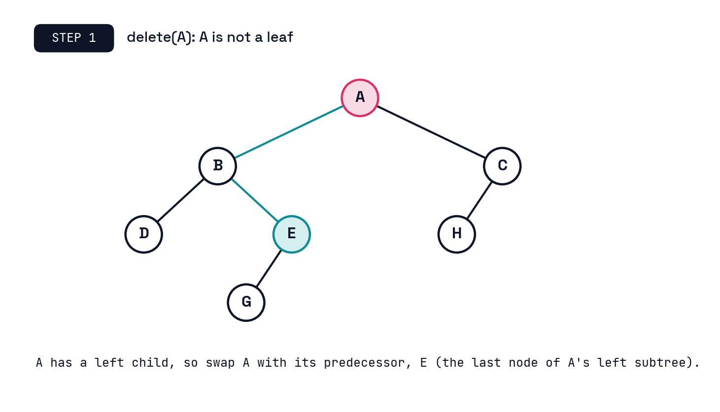
If X is a leaf, detach it from its parent. Done.
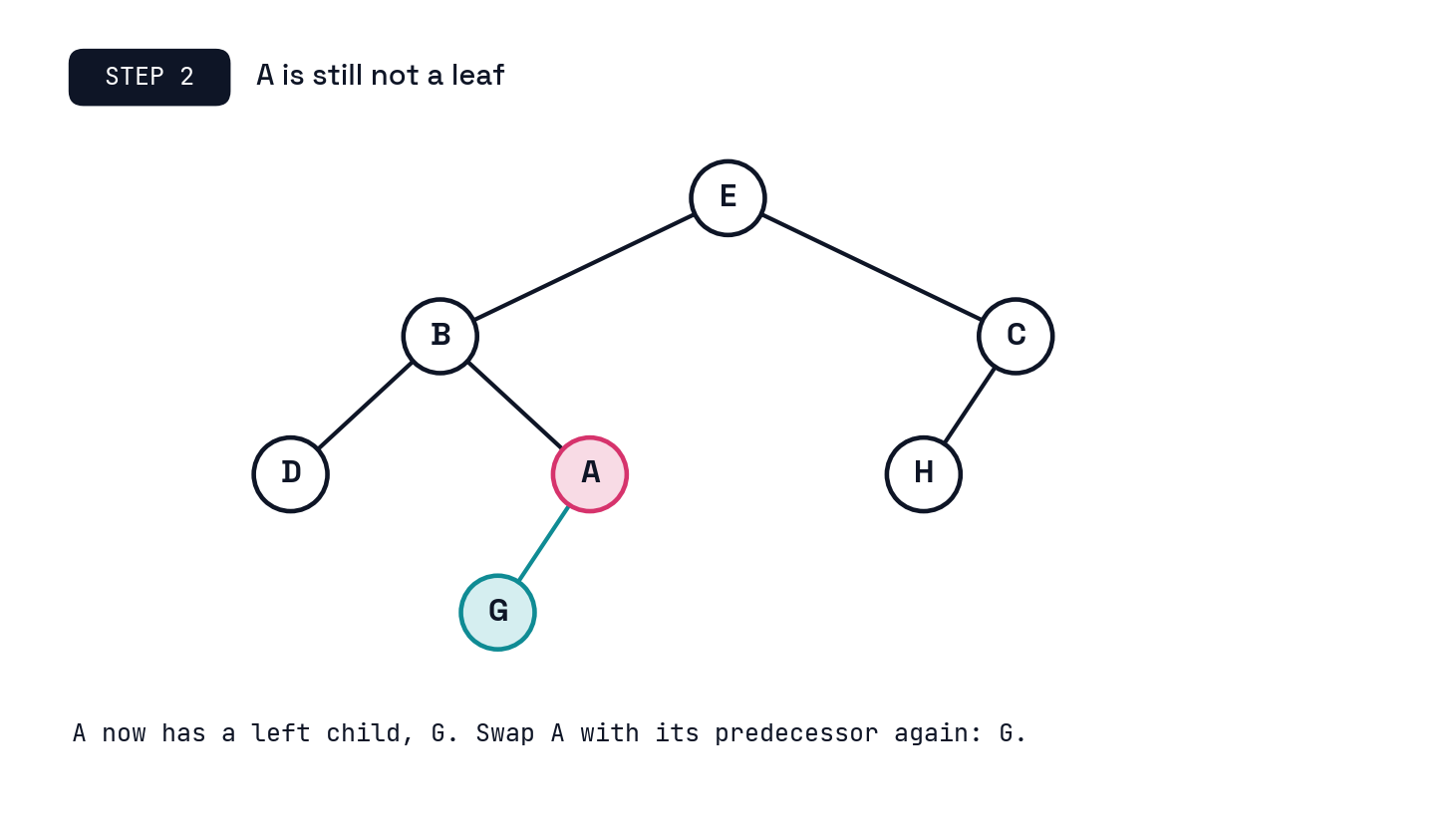
If X has a left child, swap its item with its predecessor’s item and delete from the predecessor’s node instead. The predecessor of a node with a left child is the last node of that left subtree, which has no right child, so it is closer to being a leaf.
Otherwise X has a right child: swap with the successor and recurse.
Every step moves the item one level down, so at most \(h\) swaps: \(O(h)\).

Deleting the root, in three steps

Why the swap trick is safe

Swapping a node’s item with its predecessor’s item breaks traversal order in exactly one place: those two items are now out of order with each other, and with nothing else.
Then we delete the item we wanted gone. What remains is in traversal order again, minus one item.
We never rewire anything but a leaf. That is what keeps every case \(O(1)\) pointer work on top of an \(O(h)\) walk.

Application 1: the Set

Give the order a meaning

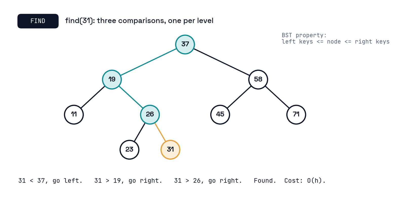
A binary search tree (BST) is a binary tree whose traversal order is increasing key order. Equivalently, the BST property: for every node, every key in its left subtree is at most its key, and every key in its right subtree is at least its key.

Same structure, same six algorithms. We have only decided where each item goes.

find(k), like binary search

The rest of the Set interface

Operation	How	Cost
`find(k)`	compare, go left or right	\(O(h)\)
`insert(x)`	`find` where it would be, then `insert_before`/`after`	\(O(h)\)
`delete(k)`	`find`, then delete the node	\(O(h)\)
`find_min`, `find_max`	`subtree_first`, `subtree_last` on the root	\(O(h)\)
`find_prev(k)`, `find_next(k)`	`find`, then `predecessor`/`successor`	\(O(h)\)
`build(X)`	sort, then build a balanced tree recursively	\(O(n \log n)\)

Every row is \(O(h)\). The goal column wanted \(O(\log n)\). So the entire question is: how big is \(h\)?

Application 2: the Sequence

The same tree, a different meaning

Now let traversal order be sequence order: the item at position \(i\) is the \(i\)-th node in traversal order.
get_at(i) by walking the whole traversal is \(O(n)\). Too slow.
If every node knew the size of its subtree, we could steer: compare \(i\) with the size of the left subtree.
Augmentation: store node.size. When a leaf is added or removed, add \(\pm 1\) to every ancestor’s size, along the \(O(h)\) path we walked anyway.

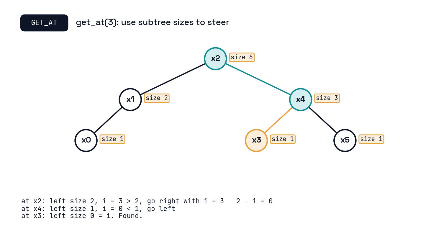
get_at(i) with subtree sizes

Steering rule

At node X with left subtree size \(n_L\):
if \(i < n_L\), recurse left with the same \(i\);
if \(i = n_L\), X is the answer;
if \(i > n_L\), recurse right with \(i' = i - n_L - 1\).
One comparison per level: \(O(h)\). Every Sequence operation (insert_at, delete_at, get_at, set_at) is then \(O(h)\) via get_at plus today’s insert or delete.
Two interfaces, one structure. Augmentation is the pattern that made the second one work; keep it in mind for the project.

The catch

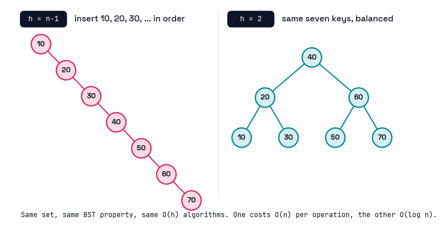
h is not log n. Not yet.

What Wednesday fixes

Insert the keys \(10, 20, 30, \ldots\) in order and a BST becomes a linked list: \(h = n - 1\), and every “\(O(h)\)” operation is \(O(n)\).
The same seven keys fit in a tree of height \(2\). The algorithms do not change; only the shape does.
Wednesday: rotations, a local \(O(1)\) rewiring that preserves traversal order, and AVL trees, which use them to keep \(h = O(\log n)\) after every insert and delete.
Then every row of both tables reads \(O(\log n)\), worst case, no randomness. That closes the gap we opened at the start of today.

Activity: trace it by hand

Your turn, in pairs

Take one worksheet per pair.

Side 1: given a drawn tree, write its traversal order, then find subtree_first, two successors, and where an insert lands.

Side 2: build a BST from a key sequence, delete its root, then find an insertion order that makes the tree as tall as possible.

10 minutes. Worksheets come in at the end; one per pair, both names on it.

Debrief: side 1

Tree: root \(M\) with left child \(G\) and right child \(T\); \(G\) has children \(C\) and \(K\); \(T\) has right child \(W\); \(K\) has left child \(J\).

Traversal order: \(C, G, J, K, M, T, W\).
subtree_first(M) \(= C\) (keep going left).
successor(G) \(=\) first of \(G\)’s right subtree \(= J\). successor(K) \(= M\) (climb: \(K \to G\) from the right, \(G \to M\) from the left).
insert_after(M, P): \(M\) has a right child, so \(P\) becomes the left child of successor(M) \(= T\).

Debrief: side 2

Insert \(41, 17, 65, 8, 30, 52, 79\) into an empty BST:

\(41\) is the root; \(17\) left, \(65\) right; \(8\) and \(30\) under \(17\); \(52\) and \(79\) under \(65\). Height \(2\), perfectly balanced.
delete(41): \(41\) has a left child, so swap with its predecessor \(30\) (the last node of the left subtree), which is a leaf; detach it. New root \(30\).
Tallest tree: any sorted or reverse-sorted order, such as \(8, 17, 30, 41, 52, 65, 79\), gives height \(6\). Total insertion cost \(0 + 1 + \cdots + 6 = 21\) comparisons, versus \(10\) for the balanced order. That gap is \(\Theta(n^2)\) versus \(\Theta(n \log n)\) in general.

HW3: analyze, build, validate

A different kind of homework

The assignment in one slide

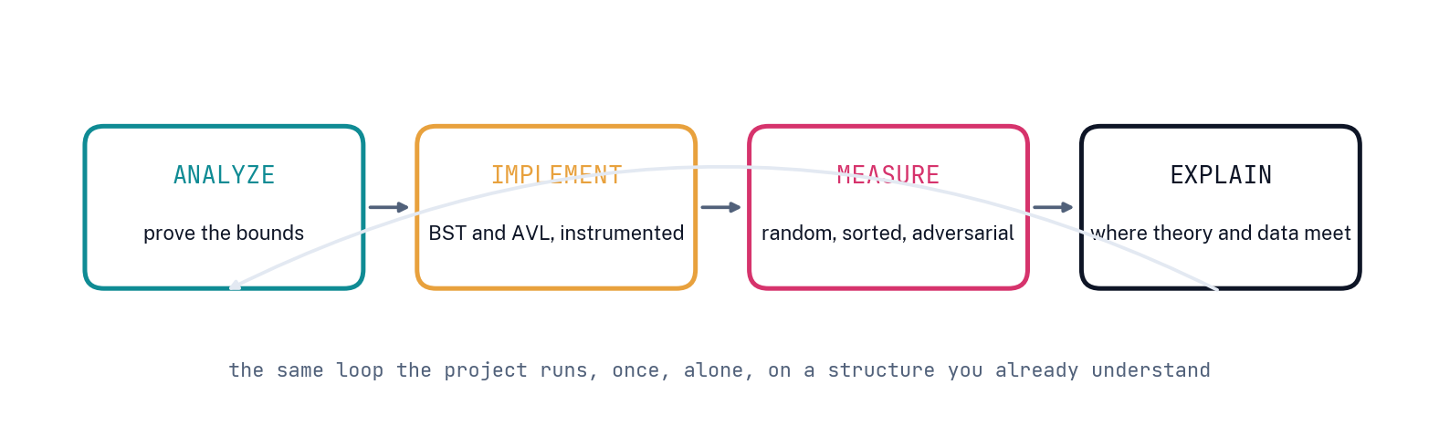
HW3: Binary Search Trees, Analyzed and Measured. Due Wednesday, September 30 at 9:59 PM. 100 points.

Analyze (35): prove the height lower bound for any binary tree, the \(\Theta(n^2)\) cost of sorted insertions, and (after Wednesday) the AVL height bound and rotation count.
Implement (30): an unbalanced BST and an AVL tree, insert, find, height, in-order traversal, with counters for comparisons and rotations. Python starter provided; any language is allowed.
Measure and explain (35): run random, sorted, and one adversarial sequence you design for \(n\) up to \(2^{16}\), write results.csv in the given format, plot height against \(\log_2 n\), and write one page on where the data and the analysis agree and where they do not.

Why this one is fun

You get to break something on purpose: build the input that makes a plain BST fall over, then watch the AVL tree shrug it off.
Your plots will show constants the analysis hides. Explaining them is the interesting part, and it is graded.
It is the project loop from this morning, run once, alone, on a structure you already understand. By Wednesday the 30th you will have done every step your team needs to do in October.
One hint: a recursive insert on a sorted sequence of \(65{,}536\) keys will exhaust Python’s default recursion limit. That is the analysis showing up in your runtime. Write insert iteratively.

Wrapping up

The one-slide version

A binary tree is three pointers per node and one rule for order: left subtree, node, right subtree. From that rule come first, last, successor, predecessor, insert-before/after, and delete, each walking one path, each \(O(h)\). Assign the order a meaning and the same tree is a Set (keys sorted, find by comparing) or a Sequence (positions, steered by subtree sizes). Everything is \(O(h)\), and \(h\) can be \(n\). Wednesday makes it \(\log n\).

What’s next

Wednesday at a glance

Topics: Binary trees, part 2. Rotations, the AVL balance rule, and why it forces \(h = O(\log n)\); how insert and delete rebalance in \(O(\log n)\) with \(O(1)\) rotations per insert.

Supplemental reading (highly recommended): CLRS Chapter 12 for today; Chapter 13 for Wednesday (CLRS treats red-black trees; the balancing idea is the same, and the AVL details are in lecture).

Upcoming deliverables:

HW2 due Wednesday, September 23 at 9:59 PM (extended).
Project teams set by Friday, September 25.
HW3 due Wednesday, September 30 at 9:59 PM; the AVL parts need Wednesday’s lecture.

References

Sources

Cormen, T. H., Leiserson, C. E., Rivest, R. L., and Stein, C. Introduction to Algorithms, 4th edition, MIT Press. Chapter 12 (Binary Search Trees); Chapter 13 (Balanced trees); Section 17.1 (Augmenting data structures).
Adelson-Velsky, G. M., and Landis, E. M. (1962). An algorithm for the organization of information. Doklady Akademii Nauk SSSR, 146, 263 to 266.
CS 351 Syllabus: Canvas.