AVL Trees

Lecture W5W1: Binary Trees, Part 2: One Tree, Two Interfaces, and Keeping It Short

Lucas P. Cordova, Ph.D.

lpcordova@willamette.edu

Willamette University

September 23, 2026

Learning objectives

What you will leave with

Separate an interface (what operations you ask for) from a storage choice (how the items are kept), and place the binary tree among the storage choices.
Explain how one tree shape serves the Set interface (organized by key) and the Sequence interface (organized by position), and what each needs stored at a node.
Define skew and the AVL property, and prove why it forces \(h = O(\log n)\).
Perform a rotation by hand, and choose between a single and a double rotation from the skews.
Trace AVL insert and delete, including the walk back up that fixes heights.

Today’s goal

Monday ended with every tree operation costing \(O(h)\) and no promise about \(h\). Today we make the promise. First, though, we sort out what the tree is for, because “one structure, two jobs” is the part that was confusing.

Two interfaces, five storage choices

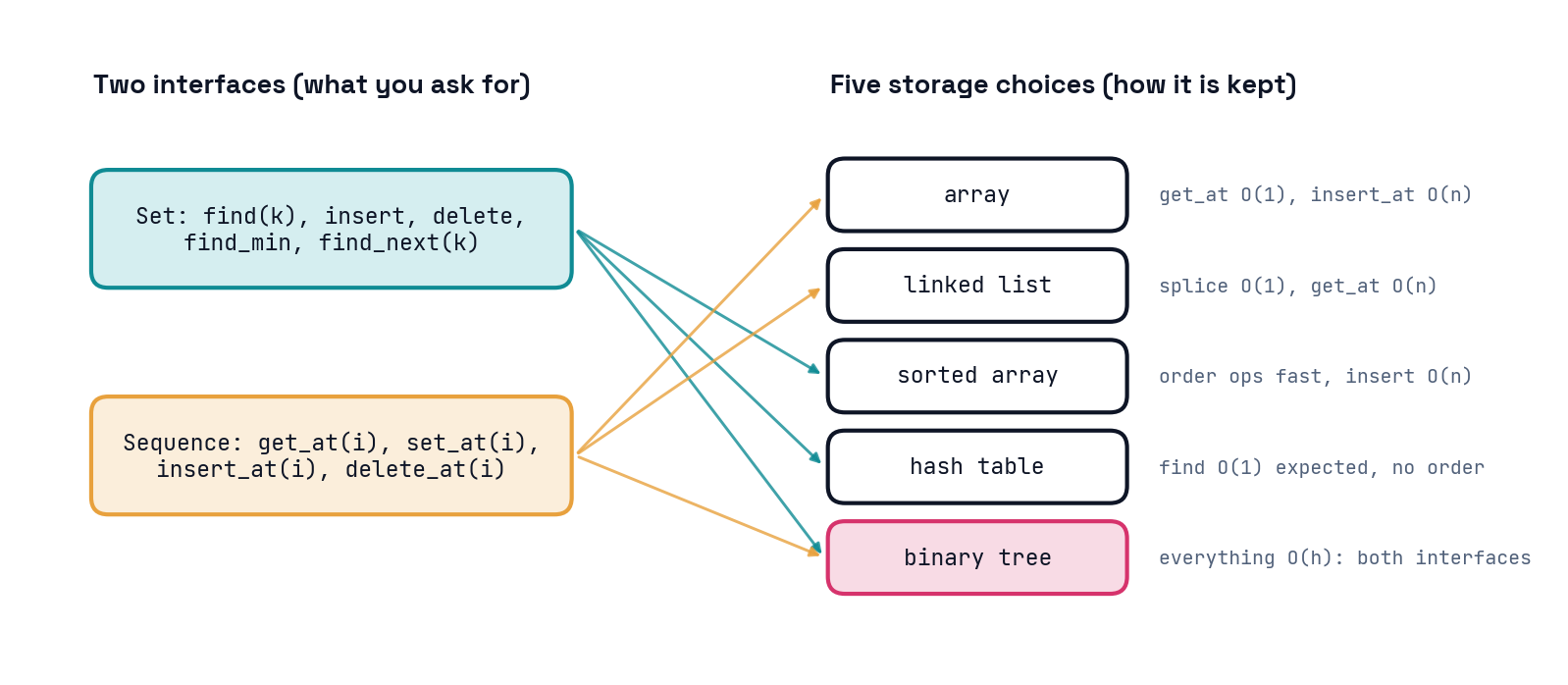
Interfaces are questions; storage is how you answer them

An interface is the list of operations a client is allowed to ask for. It says nothing about how the data is kept.
The Set interface asks about keys: find(k), insert(x), delete(k), find_min(), find_next(k). “Is 37 in here? What comes after it?”
The Sequence interface asks about positions: get_at(i), set_at(i, x), insert_at(i, x), delete_at(i). “What is the third item? Put this one fourth.”
A storage choice is a way to lay the items out in memory: array, linked list, sorted array, hash table, binary tree. Each one answers some questions cheaply and others expensively.

The map

Set interface: the storage choices so far

Operation	Sorted array	Hash table	Binary tree
`find(k)`	\(\log n\)	\(1\) (e)	\(h\)
`insert(x)`, `delete(k)`	\(n\)	\(1\) (a, e)	\(h\)
`find_min()`, `find_max()`	\(1\)	\(n\)	\(h\)
`find_prev(k)`, `find_next(k)`	\(\log n\)	\(n\)	\(h\)

(e) expected: an average over the hash function’s randomness. (a) amortized: an average over a sequence of operations, because of the occasional table doubling. Everything else is worst case.

The hash table is the fastest storage for a Set if you never ask an order question. The moment you do, it is a linear scan. The sorted array answers order questions but cannot change cheaply. The tree does everything in \(O(h)\), and \(h\) is the whole story.

Sequence interface: the storage choices so far

Operation	Array	Linked list	Binary tree
`get_at(i)`, `set_at(i, x)`	\(1\)	\(n\)	\(h\)
`insert_first`, `delete_first`	\(n\)	\(1\)	\(h\)
`insert_last`, `delete_last`	\(1\) (a)	\(n\)	\(h\)
`insert_at(i, x)`, `delete_at(i)`	\(n\)	\(n\)	\(h\)

(a) amortized: insert_last on a dynamic array is \(O(1)\) averaged over a sequence because of the occasional resize.

Arrays are fast to index and slow to splice; linked lists are the reverse. Neither does insert_at(i) in better than linear time. The tree column is the only one with no \(n\) in it. Again: everything is \(h\).

The claim of the day

One tree shape, with one set of \(O(h)\) operations from Monday, can be organized by key to serve the Set interface or organized by position to serve the Sequence interface. If we can keep \(h = O(\log n)\), it beats every other storage choice on the operations they are bad at, and ties them within a log factor on the ones they are good at.

The tree as a Set (Monday, briefly)

Organized by key

A binary search tree stores items so that traversal order is increasing key order. Equivalently, at every node, keys in the left subtree \(\leq\) node’s key \(\leq\) keys in the right subtree.

The tree decides where an item goes by comparing keys on the way down. That is the only extra thing a node needs: its key.
find(k): compare, go left or right, \(O(h)\). insert(x): find where it would be, attach a leaf. find_min: go left until you cannot. find_next(k): find, then successor.
What you get for free: find_next and find_min cost the same as find. That is the row the hash table cannot do.

Where we stopped Monday

Operation	Cost
`find(k)`, `insert(x)`, `delete(k)`	\(O(h)\)
`find_min()`, `find_max()`, `find_prev(k)`, `find_next(k)`	\(O(h)\)
`build(X)`	\(O(n \log n)\)

Every row \(O(h)\). Now the second organization, then we fix \(h\).

The tree as a Sequence

Organized by position

Same node, same pointers, same insert_after, delete, successor from Monday. No keys. The items can be anything, in any order the client chooses.
The rule: traversal order is the sequence order. The leftmost node is position 0, its successor is position 1, and so on. Position is not stored anywhere; it is where the node sits.
get_at(i) therefore asks: “which node is \(i\)-th in traversal order?” It returns that node’s item. It is not searching for a value; there is no value to search for.
Walking the traversal order to count to \(i\) costs \(O(n)\). We want \(O(h)\). So we need to be able to skip whole subtrees.

Store one extra number per node

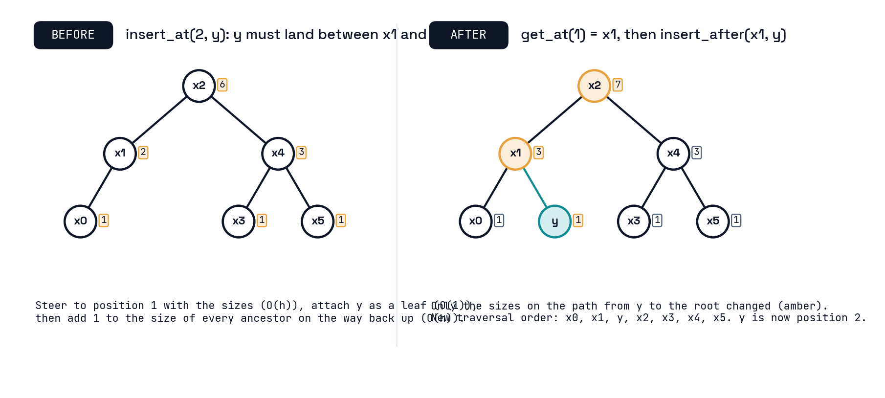
Augmentation: each node also stores size, the number of nodes in its subtree (itself included). A leaf has size 1; a node’s size is 1 plus its children’s sizes.

With sizes, a node knows how many items come before it within its own subtree: exactly the size of its left subtree, \(n_L\).
So at any node, the node itself is at local position \(n_L\). Everything in the left subtree is at positions \(0\) to \(n_L - 1\); everything in the right subtree starts at position \(n_L + 1\).
That is enough to steer, like binary search, without ever comparing values.

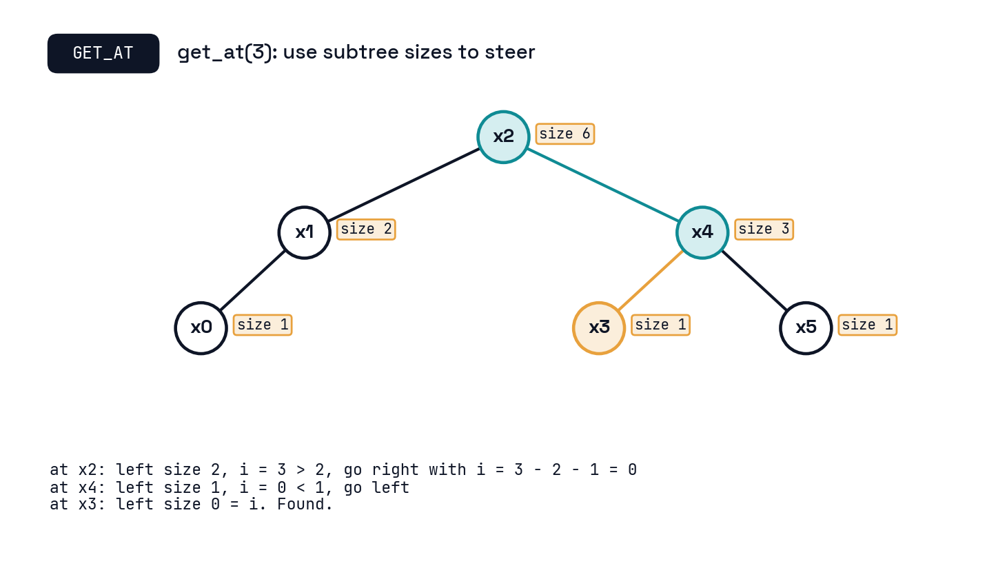
Steering rule for get_at(i)

At node X with left-subtree size \(n_L\):

if \(i < n_L\): the answer is in the left subtree; recurse left with the same \(i\).
if \(i = n_L\): X is the answer.
if \(i > n_L\): the answer is in the right subtree; recurse right with \(i' = i - n_L - 1\), because you just skipped \(n_L\) left items plus X itself.
One comparison per level: \(O(h)\).

Worked example: get_at(3)

Keeping the sizes correct

The rest of the Sequence interface

Operation	How	Cost
`get_at(i)`, `set_at(i, x)`	steer by sizes	\(O(h)\)
`insert_at(i, x)`	`get_at(i)`, then `insert_before`; add 1 to sizes on the path up	\(O(h)\)
`delete_at(i)`	`get_at(i)`, then delete; subtract 1 on the path up	\(O(h)\)
`insert_first`, `insert_last`, and their deletes	`subtree_first`/`subtree_last`, then the above	\(O(h)\)
`build(X)`	build a balanced tree from the list directly	\(O(n)\)

Same shape, same \(O(h)\), one integer per node. The Set stores a key and compares; the Sequence stores a size and counts.

Side by side

	Tree as a Set	Tree as a Sequence
Organized by	key	position in traversal order
Extra field per node	`key`	`size`
How `find` / `get_at` steers	compare \(k\) with `node.key`	compare \(i\) with `node.left.size`
What must stay true after every change	BST property	sizes on the changed path
Cost of everything	\(O(h)\)	\(O(h)\)

Which brings us, for the last time, to \(h\).

The problem with h

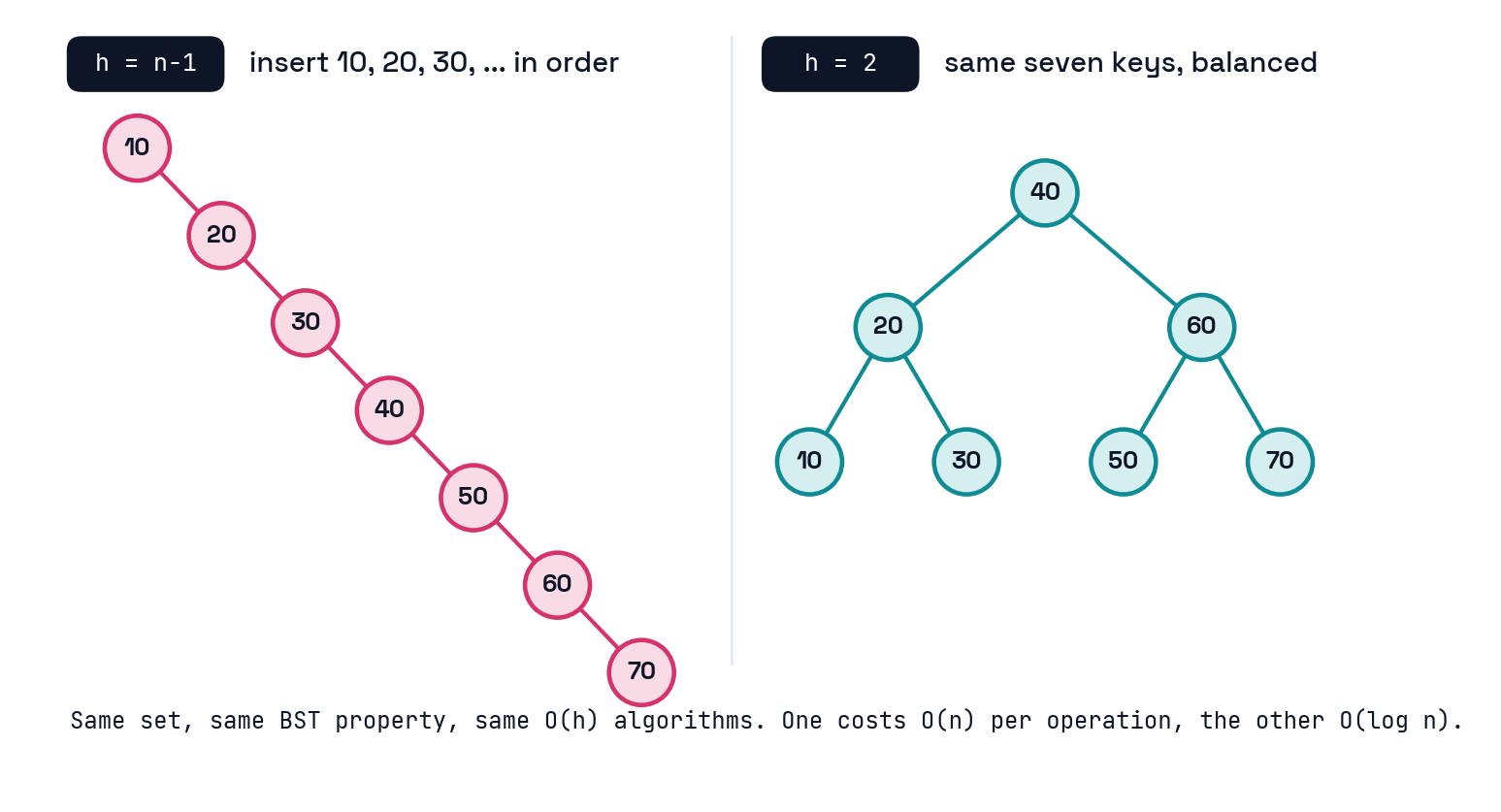
Same keys, two heights

What we need

Insert keys in sorted order and a BST is a chain: \(h = n - 1\). Every “\(O(h)\)” is \(O(n)\), and we are no better than a linked list.
The lower bound from HW3: any binary tree with \(n\) nodes has \(h \geq \log_2(n+1) - 1\). So \(\Theta(\log n)\) is the best we can hope for.
The plan: after every insert and delete, spend \(O(\log n)\) extra work to push the tree back toward balanced. The fix must preserve traversal order, or it would break both the Set and the Sequence.
The tool is a rotation. The rule that says when to use it is the AVL property. Together: Adelson-Velsky and Landis, 1962.

Rotations

One local move

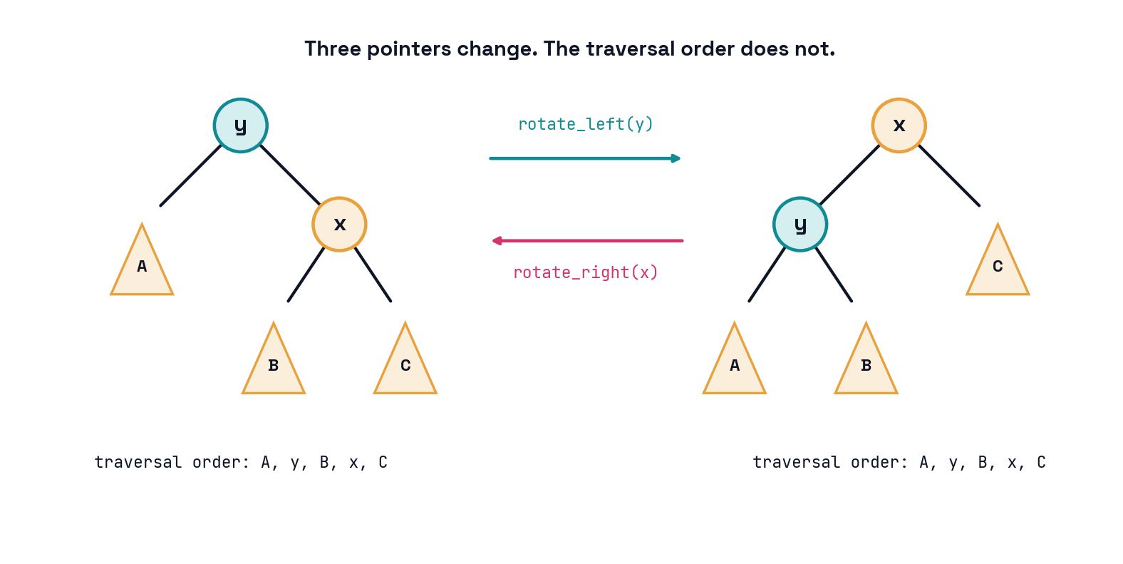
What a rotation does and does not do

rotate_left(y): y’s right child x moves up to y’s place; y becomes x’s left child; x’s old left subtree B becomes y’s right subtree.
Three pointers change (plus parents). \(O(1)\) time, no search, no comparisons.
Traversal order before: \(A, y, B, x, C\). After: \(A, y, B, x, C\). Identical. So the BST property survives, and so does sequence order.
Heights change for exactly two nodes, x and y. Sizes too, if you keep them. Everything else is untouched.
rotate_right is the mirror image. Rotations are the only way we will ever move a node that is not a leaf.

Quick check 🤔

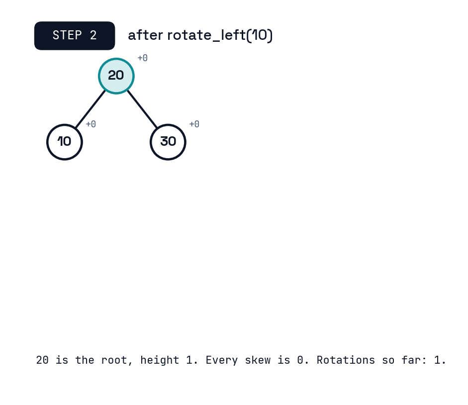
Rotate left at the root of the chain \(10 \to 20 \to 30\). What is the new root? \(20\), with \(10\) and \(30\) as children: height drops from \(2\) to \(1\).
Rotate left at the root of a perfectly balanced tree of seven keys. Did the height go up or down? Up, by one. Rotations are not automatically good; they have to be aimed.

The AVL property

Skew

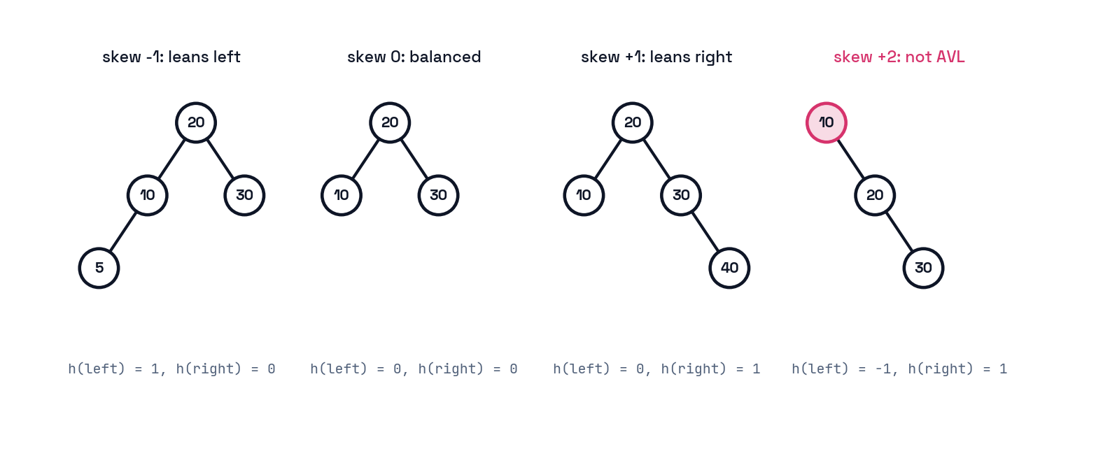
The skew of a node is \(h(\text{right}) - h(\text{left})\), where an empty subtree has height \(-1\). A node is balanced if its skew is \(-1\), \(0\), or \(+1\). A tree is AVL if every node is balanced.

Why “within one” is enough

Let \(N(h)\) be the fewest nodes an AVL tree of height \(h\) can have. Fewest nodes for a given height is the worst case for us.
\(N(0) = 1\), \(N(1) = 2\). For \(h \geq 2\): one subtree has height \(h - 1\), the other at least \(h - 2\), so \(N(h) = 1 + N(h-1) + N(h-2)\).
Drop the \(1\) and the taller term: \(N(h) \geq 2\,N(h-2)\), so \(N(h) \geq 2^{h/2}\).
An AVL tree with \(n\) nodes therefore has \(n \geq 2^{h/2}\), that is, \(h \leq 2 \log_2 n\).
The exact solution is Fibonacci-shaped and gives \(h \leq 1.44 \log_2 n\). HW3 Problem 2 asks you to write this out.

The one-slide version so far

If every node’s subtrees differ in height by at most one, the tree’s height is \(O(\log n)\). So: keep that true after every change, and every \(O(h)\) row in both tables becomes \(O(\log n)\).

Insert

The algorithm

Insert as a leaf exactly as before (BST: by key; Sequence: by position). \(O(h)\).
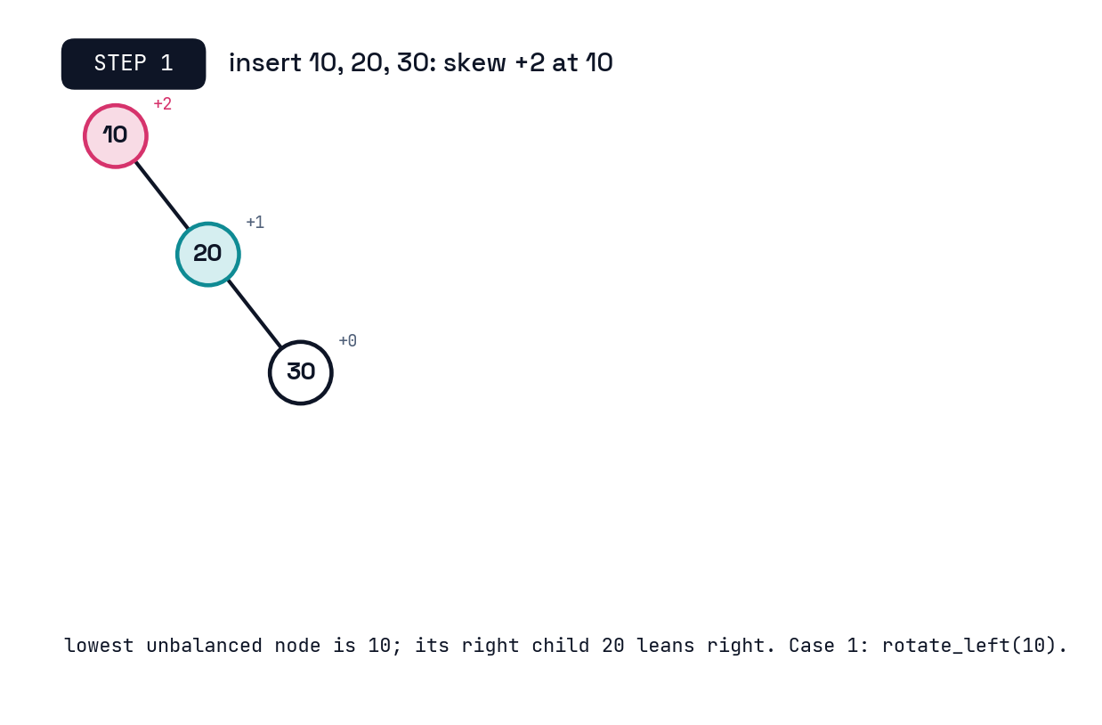
Walk up from the new leaf to the root. At each node, recompute height (and size) from the children. \(O(1)\) per node.
The first node whose skew becomes \(\pm 2\) is the lowest unbalanced node. Fix it with one or two rotations, chosen by the shape below it.
Keep walking up, recomputing heights. Nothing else will be unbalanced (next section says why).

Two shapes, two fixes

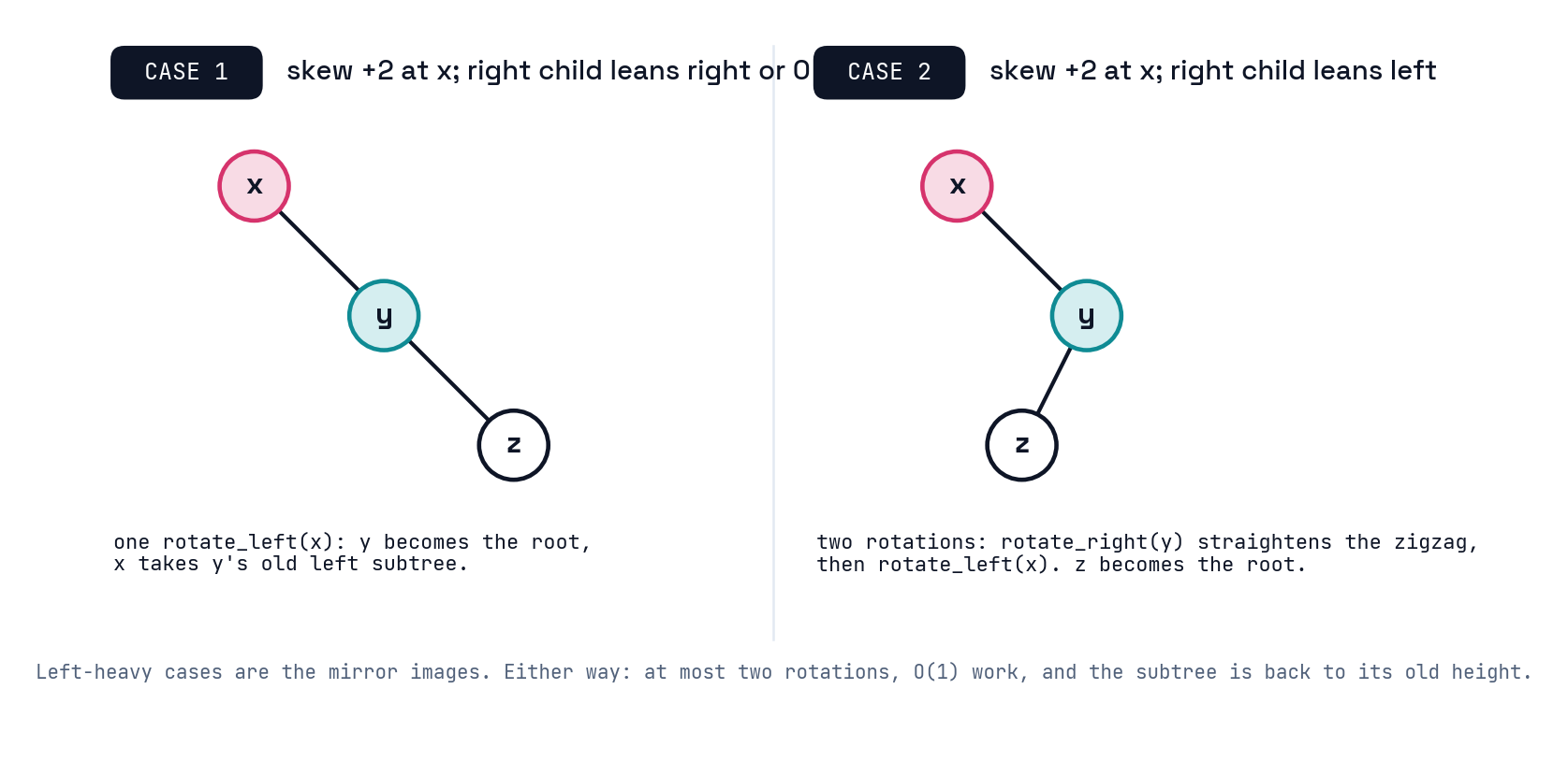
Reading the shape from the skews

Let x be the lowest unbalanced node.

skew(x) = +2 (right-heavy). Look at x.right:
- skew \(\geq 0\): single rotate_left(x).
- skew \(= -1\): double: rotate_right(x.right), then rotate_left(x).
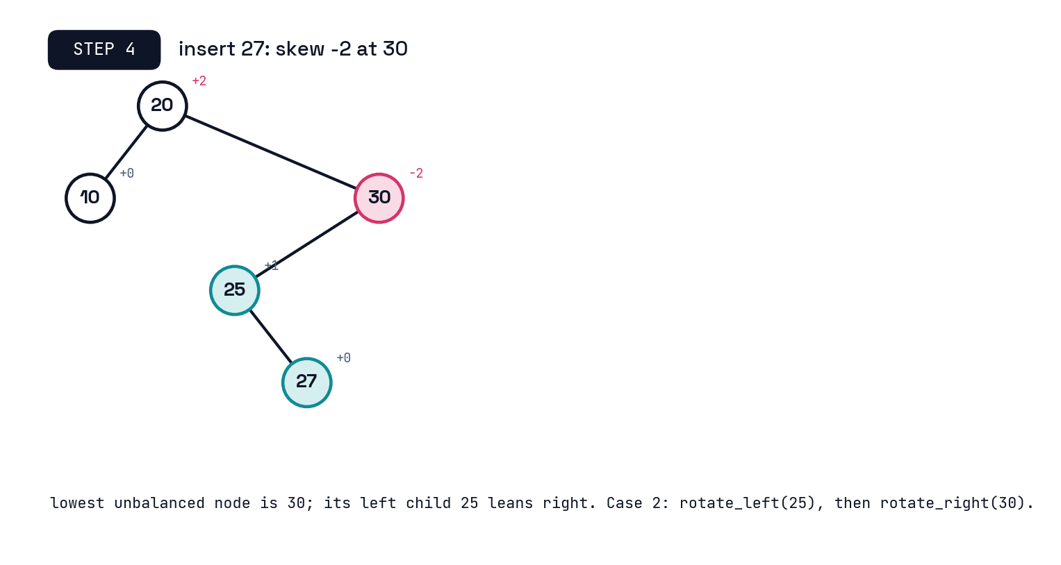
skew(x) = -2 (left-heavy). Look at x.left:
- skew \(\leq 0\): single rotate_right(x).
- skew \(= +1\): double: rotate_left(x.left), then rotate_right(x).
The rule of thumb: if the heavy grandchild is on the same side as the heavy child, one rotation; if it zigzags, straighten it first.

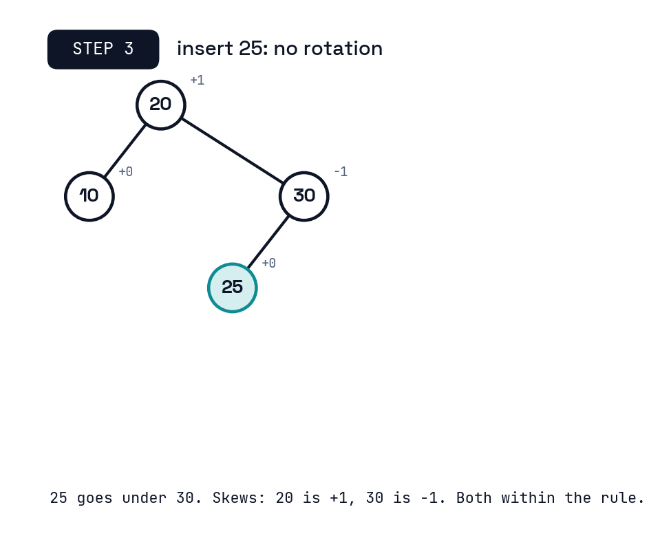
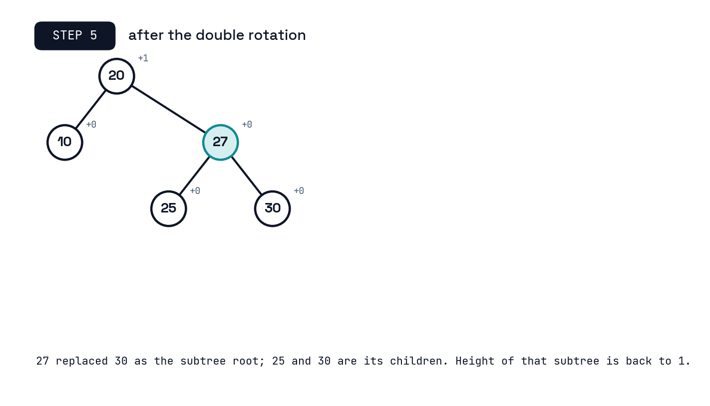
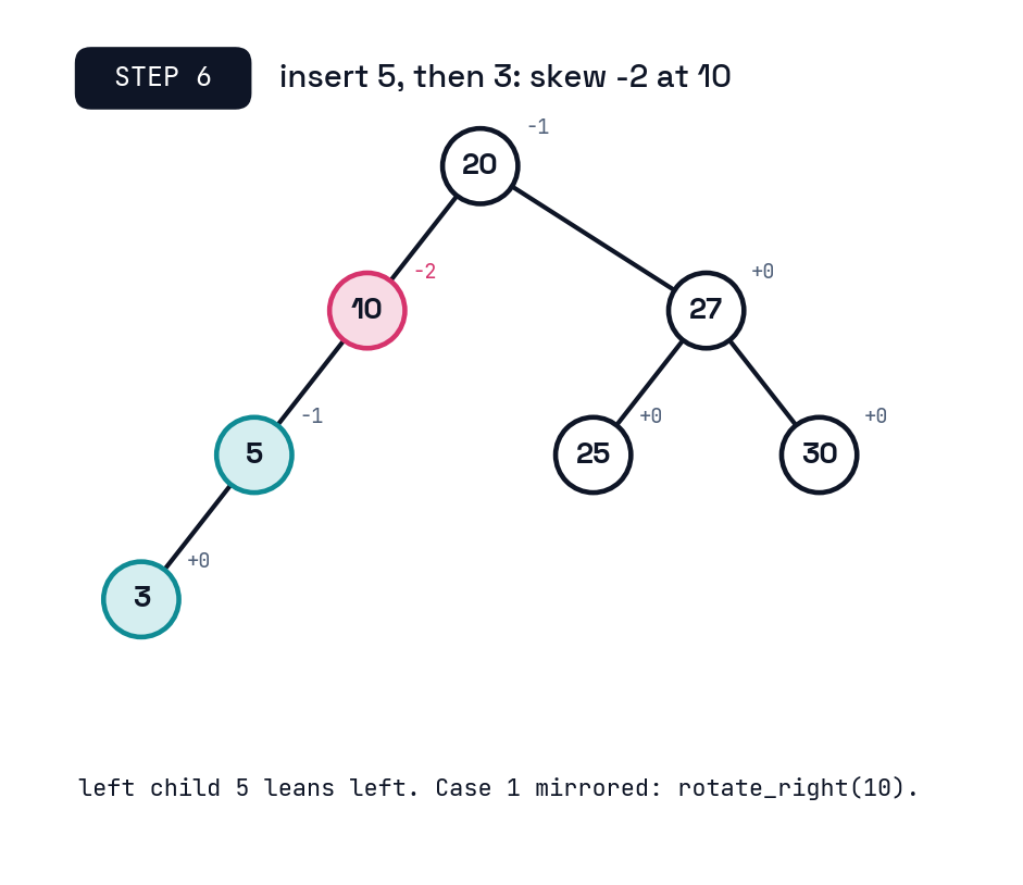
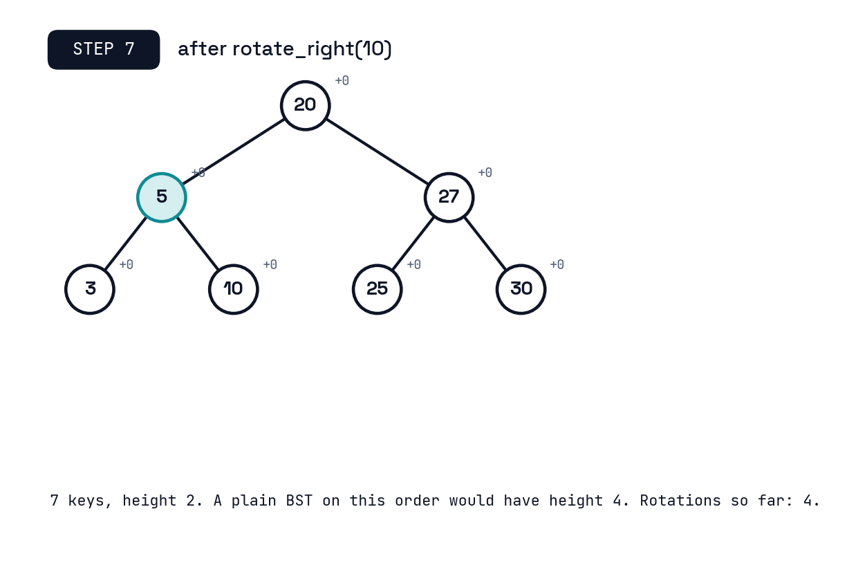
Walkthrough: 10, 20, 30, 25, 27, 5, 3

Watch it happen

Every rotation in the walkthrough, animated: courses.lucascordova.phd/dsaviz

Insert the keys \(10, 20, 30, 25, 27, 5, 3\) in that order and step through; the tool names each rotation as it performs it, and the label next to each node is its height (skew), for example 2 (+1), using today’s conventions (leaf height \(0\), skew \(= h(\text{right}) - h(\text{left})\)).
Then try the sorted sequence \(1, 2, 3, \ldots, 15\) and watch the tree stay at height \(3\).

Why one fix per insert is enough

Before the insert, the lowest unbalanced node x had height \(k + 1\) (tall side \(k\), short side \(k - 1\)).
The insert made the tall side \(k + 1\). After the single or double rotation, the subtree that replaces x has both sides at height \(k\), so its height is \(k + 1\) again.
Every ancestor of x now sees exactly the subtree height it saw before the insert. Their skews are unchanged, so they are still balanced.
Total: one path down, one path up, at most two rotations. \(O(\log n)\).

Delete

Almost the same walk

Delete as on Monday: swap down to a leaf, detach it. \(O(h)\).
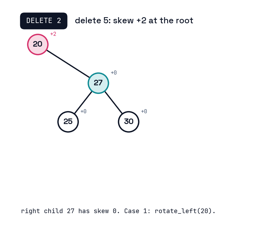
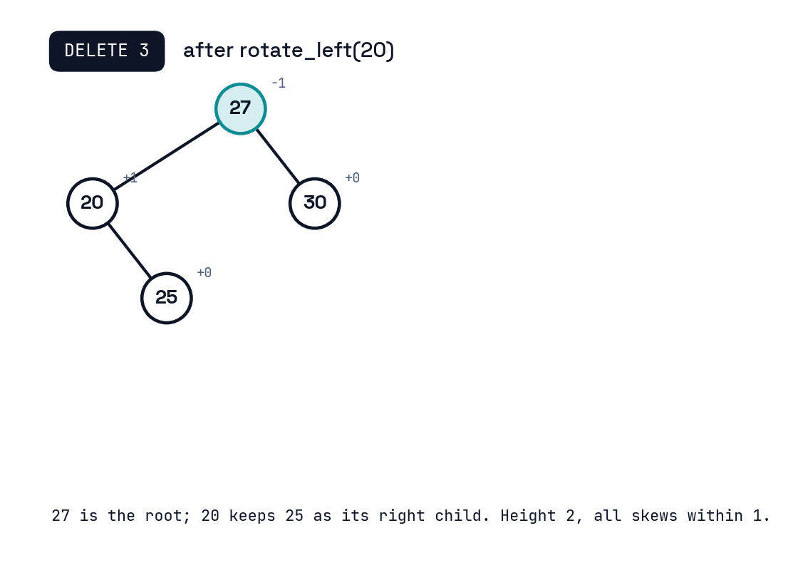
Walk up from the detached leaf’s parent, recompute heights, rotate at any node whose skew hits \(\pm 2\), using the same two shapes.
One difference: a deletion can shrink a subtree, and a rotation that fixes the lowest node can shrink it again, so the imbalance can propagate upward. You may rotate at several ancestors.
Still at most two rotations per level, still one path: \(O(\log n)\).

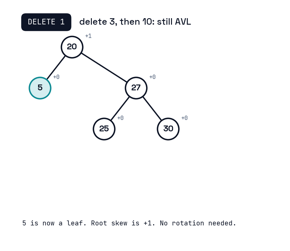
Walkthrough: delete 3, 10, then 5

The tables, finished

Set interface	Sorted array	Hash table	AVL tree
`find(k)`	\(\log n\)	\(1\) (e)	\(\log n\)
`insert(x)`, `delete(k)`	\(n\)	\(1\) (a, e)	\(\log n\)
`find_min`, `find_max`, `find_prev`, `find_next`	\(\log n\) or \(1\)	\(n\)	\(\log n\)

Sequence interface	Array	Linked list	AVL tree
`get_at(i)`, `set_at(i, x)`	\(1\)	\(n\)	\(\log n\)
`insert_at(i, x)`, `delete_at(i)`	\(n\)	\(n\)	\(\log n\)

(e) expected, (a) amortized, as before. The AVL column has neither.

Worst case, no randomness, no amortization. That is the promise Monday could not make.

Activity: keep it balanced

Your turn, in pairs

Take one worksheet per pair.

Side 1: insert a sequence of keys into an empty AVL tree, drawing the tree after each insert and naming every rotation you perform.

Side 2: delete three keys from the resulting tree, one at a time, with the same bookkeeping, then answer two questions about heights.

12 minutes. Worksheets come in at the end; one per pair, both names on it.

Do it on paper first, then check yourselves: dsaviz AVL tree

Debrief: side 1

Insert \(50, 30, 70, 20, 40, 10, 45, 42\):

\(50, 30, 70, 20, 40\): no rotations. Root \(50\), height \(2\).
\(10\): skew \(-2\) at \(50\); left child \(30\) has skew \(-1\) (same side). Single rotate_right(50). New root \(30\), children \(20\) (with \(10\)) and \(50\) (with \(40\), \(70\)). Height \(2\).
\(45\): goes right of \(40\). Skews: \(40\) is \(+1\), \(50\) is \(0\), \(30\) is \(+1\). No rotation. Height \(3\).
\(42\): goes left of \(45\). Now \(40\) has skew \(+2\) and its right child \(45\) has skew \(-1\): zigzag. Double: rotate_right(45), then rotate_left(40). \(42\) takes \(40\)’s place with children \(40\) and \(45\).
Final tree: \(30\) over \(20\) (\(10\)) and \(50\) (\(42\) with \(40\), \(45\); and \(70\)). Height \(3\), three single rotations in total.

Debrief: side 2

From the final tree, delete \(10\), then \(20\), then \(70\):

Delete \(10\): \(20\) is a leaf, so \(30\) has left height \(0\) and right height \(2\): skew \(+2\). Right child \(50\) has skew \(-1\) (its left subtree \(42\) is taller than \(70\)): zigzag. Double: rotate_right(50), then rotate_left(30). New root \(42\) with \(30\) (\(20\), \(40\)) and \(50\) (\(45\), \(70\)). Height \(2\).
Delete \(20\): \(30\) keeps \(40\) on its right, skew \(+1\). No rotation.
Delete \(70\): \(50\) keeps \(45\) on its left, skew \(-1\). No rotation.
Five keys, height \(2\), and \(\lceil \log_2 6 ceil - 1 = 2\), so no binary tree on five keys is shorter. Notice that the deletion of \(10\) needed a rotation at the root, two levels above the leaf that left.

Wrapping up

The one-slide version

The binary tree is a storage choice that serves two interfaces: organize it by key and it is a Set, organize it by position (with a size per node) and it is a Sequence. Everything costs \(O(h)\). The AVL property, every node’s subtrees within one in height, forces \(h \leq 1.44 \log_2 n\), and rotations, which rewire three pointers without touching traversal order, restore that property after any insert or delete in \(O(\log n)\). Result: every operation of both interfaces in \(O(\log n)\), worst case.

For HW3

Problem 2 is today’s height proof and the “one fix per insert” argument, written out.
Problem 3’s AVL implementation is today’s insert algorithm: attach the leaf, walk up, update heights, rotate at the lowest unbalanced node. You do not need delete.
Count single rotations; a double counts as two. Your Problem 4 data will show rotations per insert well under the bound of \(2\).

What’s next

Monday at a glance

Topics: Binary heaps and priority queues. A tree stored in an array with no pointers at all, which gives up find to make insert and delete_max cheap and simple. Then heap sort, our third \(O(n \log n)\) sort.

Supplemental reading (highly recommended): CLRS Chapter 13 for today (red-black trees are CLRS’s balanced tree; the balancing idea is the same); Chapter 6 for Monday.

Upcoming deliverables:

HW2 due tonight, 9:59 PM.
Project teams set by Friday, September 25.
HW3 due Wednesday, September 30 at 9:59 PM.

References

Sources

Cormen, T. H., Leiserson, C. E., Rivest, R. L., and Stein, C. Introduction to Algorithms, 4th edition, MIT Press. Chapter 12 (Binary Search Trees); Chapter 13 (Red-Black Trees); Section 17.1 (Dynamic order statistics).
Adelson-Velsky, G. M., and Landis, E. M. (1962). An algorithm for the organization of information. Doklady Akademii Nauk SSSR, 146, 263 to 266.
CS 351 Syllabus: Canvas.