Lecture 13: Advanced Query Techniques

DATA 351: Data Management with SQL

Lucas P. Cordova, Ph.D.

lpcordova@willamette.edu

Willamette University

March 30, 2026

What You’ll Learn This Week

Learning Objectives

By the end of this week, you will be able to:

Write subqueries in WHERE, FROM, and SELECT clauses to filter, preprocess, and compute values
Distinguish between correlated and uncorrelated subqueries and explain their performance implications
Use IN and EXISTS subquery expressions to test membership across tables
Apply LATERAL joins for per-row subquery evaluation
Construct Common Table Expressions (CTEs) for readable, maintainable queries
Generate cross tabulations with crosstab() and reclassify data using CASE

Part 1: Setting Up

Database Setup

Create and Populate the Database

Create a fresh database for this lecture:

CREATE DATABASE advanced_queries;

Download the CSV files from advanced_queries_csvs.zip ↓ and unzip them into the /tmp (macOS) or C:\Users\Public (Windows) directory.

Connect to advanced_queries database, then run the setup script provided: advanced_queries.sql ↓

Data Overview and Expected Counts

The script creates and loads the following tables:

Table	Rows	Description
`us_counties_pop_est_2019`	3,142	County population estimates
`cbp_naics_72_establishments`	2,764	Food/accommodation businesses per county
`employees`	6	Small HR demo table
`teachers`	6	Small demo table (from Ch 7)
`ice_cream_survey`	200	Office ice cream flavor preferences
`temperature_readings`	1,077	Daily temps at three stations

Verify Your Setup

SELECT count(*) FROM us_counties_pop_est_2019;     -- 3,142
SELECT count(*) FROM cbp_naics_72_establishments;  -- 3,074
SELECT count(*) FROM employees;                    -- 6
SELECT count(*) FROM ice_cream_survey;             -- 200
SELECT count(*) FROM temperature_readings;         -- 1,077

If any count is wrong, re-run the setup. We need all of these this week.

Part 2: Subqueries

A query inside a query. It’s queries all the way to town. 🛣️

What Is a Subquery?

The Big Picture

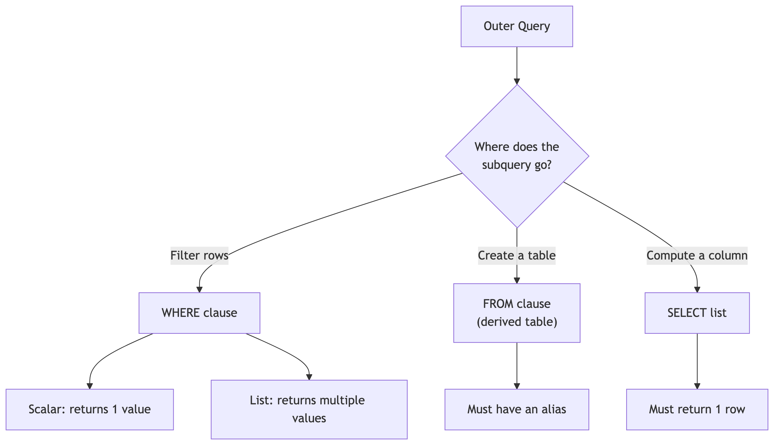
A subquery is a query nested inside another query, enclosed in parentheses.

Subqueries can:

Generate values for filtering (WHERE)
Create temporary tables (FROM)
Compute columns (SELECT)

Subquery Process

Subquery Types

There are two types of subqueries:

Correlated: references the outer query, runs once per row
Uncorrelated: runs once, independent of outer query

Subqueries can also be scalar or non-scalar.

Scalar: returns a single value
Non-scalar: returns multiple values (list)

Filtering with Subqueries in WHERE

Scalar Subquery in WHERE

The most common pattern: use a subquery to compute a threshold, then filter on it. Run this. Inner query first, outer query second. What is this telling us ❓🤔

SELECT county_name,
       state_name,
       pop_est_2019
FROM us_counties_pop_est_2019
WHERE pop_est_2019 >= (
    SELECT percentile_cont(.9) WITHIN GROUP (ORDER BY pop_est_2019)
    FROM us_counties_pop_est_2019
)
ORDER BY pop_est_2019 DESC;

The inner query computes the 90th percentile of county populations. The outer query returns only counties at or above that threshold.
The subquery executes first, returns a single value (213,707.3), and the outer query uses it like a constant. This is a scalar subquery and it’s uncorrelated: it runs exactly once.

How It Executes

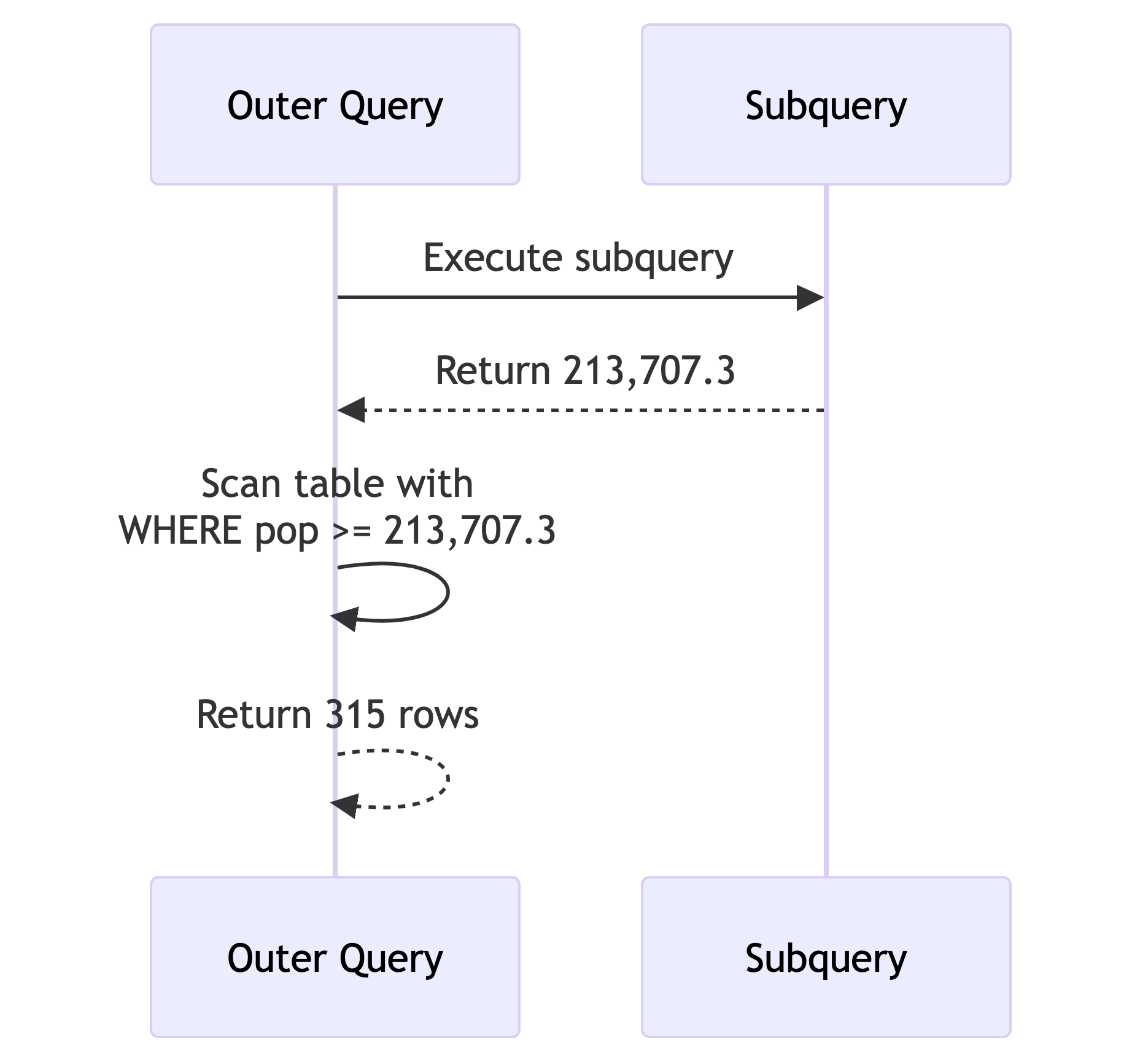
Key points:

The subquery runs once before the outer query starts scanning
The result (213,707.3) acts like a constant
315 rows returned (about 10% of 3,142)

Note: Using percentile_cont() in a subquery only works with a single input. Passing an array would return an array, and the >= comparison would fail.

Subquery with DELETE

Subqueries work with DML too. Let’s create a copy and prune it Run this.:

CREATE TABLE us_counties_2019_top10 AS
SELECT * FROM us_counties_pop_est_2019;

DELETE FROM us_counties_2019_top10
WHERE pop_est_2019 < (
    SELECT percentile_cont(.9) WITHIN GROUP (ORDER BY pop_est_2019)
    FROM us_counties_2019_top10
);

SELECT count(*) FROM us_counties_2019_top10;

You started with 3,142 counties and now have ~315 (the top 10%).
In a pipeline context: this is how you build filtered summary tables. You copy the source, delete what you don’t need, keep the rest for downstream consumers.

🧠 Quick Check: Subquery Execution

When does an uncorrelated subquery in a WHERE clause execute?

A. Once before the outer query starts
B. Once per row of the outer query
C. After the outer query finishes
D. It depends on the table size

A. The database computes the inner value once, then scans the outer table. Correlated subqueries (coming up soon) are different: they run once per row. That distinction matters for performance.

Creating Derived Tables with Subqueries

Subquery as a Table in FROM

A subquery in the FROM clause creates a derived table: a temporary result set you can query like a regular table (run this):

SELECT round(calcs.average, 0) AS average,
       calcs.median,
       round(calcs.average - calcs.median, 0) AS median_average_diff
FROM (
    SELECT avg(pop_est_2019) AS average,
           percentile_cont(.5)
               WITHIN GROUP (ORDER BY pop_est_2019)::numeric AS median
    FROM us_counties_pop_est_2019
) AS calcs;

The inner query computes two aggregates. The outer query calculates the difference. The AS calcs alias is required: PostgreSQL demands that derived tables have names.
The average is ~104,468 and the median is ~25,726. That 78,742 gap tells us some massive counties are inflating the average. This is why we always check both.

Joining Two Derived Tables

This is powerful for combining aggregations from different tables Run this. What are your observations on what this is telling us?

SELECT census.state_name AS st,
       census.pop_est_2018,
       est.establishment_count,
       round((est.establishment_count / census.pop_est_2018::numeric) * 1000, 1)
           AS estabs_per_thousand
FROM
    (SELECT st, sum(establishments) AS establishment_count
     FROM cbp_naics_72_establishments
     GROUP BY st) AS est
JOIN
    (SELECT state_name, sum(pop_est_2018) AS pop_est_2018
     FROM us_counties_pop_est_2019
     GROUP BY state_name) AS census
ON est.st = census.state_name
ORDER BY estabs_per_thousand DESC;

Key Points on Previous Query

Each derived table aggregates to the state level separately, then they join on state name.
Tourism hotspots like DC, Montana, and Vermont top the list.
Mississippi and Kentucky are at the bottom.

🧠 Quick Check: Derived Table Rules

What happens if you forget the AS alias on a derived table?

A. PostgreSQL infers a name automatically
B. You get a syntax error
C. It works but you can’t reference the columns
D. The query runs but returns wrong results

B. PostgreSQL requires every derived table to have an alias. AS calcs, AS est, AS census: pick a name. Without it, the parser rejects the query before it even tries to run.

Generating Columns with Subqueries

Column-Level Subqueries

You can put a subquery directly in the SELECT list to add a computed column:

SELECT county_name,
       state_name AS st,
       pop_est_2019,
       (SELECT percentile_cont(.5) WITHIN GROUP (ORDER BY pop_est_2019)
        FROM us_counties_pop_est_2019) AS us_median
FROM us_counties_pop_est_2019;

Every row gets the same median value (25,726) alongside its own population. This lets you compare each county to the national benchmark without a JOIN.

On its own, that repeating value isn’t thrilling. Let’s make it useful.

Subquery in a Calculation

Take it further: compute the difference from the median inline:

SELECT county_name,
       state_name AS st,
       pop_est_2019,
       pop_est_2019 - (SELECT percentile_cont(.5) WITHIN GROUP (ORDER BY pop_est_2019)
                        FROM us_counties_pop_est_2019) AS diff_from_median
FROM us_counties_pop_est_2019
WHERE (pop_est_2019 - (SELECT percentile_cont(.5) WITHIN GROUP (ORDER BY pop_est_2019)
                        FROM us_counties_pop_est_2019))
       BETWEEN -1000 AND 1000;

This finds ~78 counties whose population is within 1,000 of the national median.

Notice the subquery appears twice: once in SELECT, once in WHERE. That redundancy is a code smell. 🦨💨

CTEs will fix it later. Hang tight.

Try It: Above-Average Counties 🎯

Write a query that returns all counties where pop_est_2019 is above the national average. Show county name, state, and population. Order by population descending.

How many counties are above average? Hint: it’s less than half. Why?

-- Your query here

SELECT county_name, state_name, pop_est_2019
FROM us_counties_pop_est_2019
WHERE pop_est_2019 > (
    SELECT avg(pop_est_2019) FROM us_counties_pop_est_2019
)
ORDER BY pop_est_2019 DESC;

Far fewer than half! The mean is pulled up by massive counties (LA, Cook, Harris), so most counties fall below average.

Key Points on Previous Query

⚠️ Median vs. mean: it matters every time.

Part 3: Subquery Expressions

Checking membership across tables. The SQL equivalent of “are you on the VIP guest list?” 🎫

IN and EXISTS

Setup: Employees and Retirees

CREATE TABLE retirees (
    id int,
    first_name text,
    last_name text
);

INSERT INTO retirees
VALUES (2, 'Janet', 'King'),
       (4, 'Michael', 'Taylor');

Now we have two employees who retired. Let’s find them, and find who’s still active.

Generating Values for IN

SELECT first_name, last_name
FROM employees
WHERE emp_id IN (
    SELECT id FROM retirees
)
ORDER BY emp_id;

IN checks if emp_id matches any value in the subquery result. Simple, readable, uncorrelated.

⚠️ Warning: Avoid NOT IN with subqueries. If the subquery returns any NULL values, NOT IN returns zero rows. Always. PostgreSQL’s own wiki recommends using NOT EXISTS instead.

Using EXISTS (Correlated)

SELECT first_name, last_name
FROM employees
WHERE EXISTS (
    SELECT id
    FROM retirees
    WHERE id = employees.emp_id
);

EXISTS returns TRUE if the subquery finds at least one row. The subquery references employees.emp_id from the outer query, making it correlated: it runs once per row.

For small tables, IN and EXISTS perform identically. For large tables, EXISTS can be faster because it short-circuits: it stops scanning as soon as it finds one match.

NOT EXISTS: The Anti-Join

SELECT first_name, last_name
FROM employees
WHERE NOT EXISTS (
    SELECT id
    FROM retirees
    WHERE id = employees.emp_id
);

Run this. Returns employees who are NOT retirees. This is an anti-join: “give me everything in table A that has no match in table B.”

O==O Pipeline use case: find new records that haven’t been processed yet.

WHERE NOT EXISTS (SELECT 1 FROM processed WHERE processed.id = raw.id)

This pattern shows up constantly in ETL workflows.

🧠 Quick Check: IN vs EXISTS

For a table with 10 million rows, which is typically faster for membership checks?

A. IN (always)
B. EXISTS (always)
C. EXISTS (usually, because it short-circuits)
D. They’re always identical

C. EXISTS stops at the first match. IN materializes the full subquery result into a list. For large datasets, that difference matters. But the optimizer is smart and sometimes rewrites one to the other. Profile, don’t guess.

Part 4: LATERAL Joins

The most powerful subquery pattern you’ve (probably) never heard of.

Using Subqueries with LATERAL

LATERAL in FROM: Reusing Calculations

LATERAL lets a subquery in the FROM clause reference columns from preceding tables. Think of it as “for each row, compute this” Run this.

SELECT county_name,
       state_name,
       pop_est_2018,
       pop_est_2019,
       raw_chg,
       round(pct_chg * 100, 2) AS pct_chg
FROM us_counties_pop_est_2019,
     LATERAL (SELECT pop_est_2019 - pop_est_2018 AS raw_chg) rc,
     LATERAL (SELECT raw_chg / pop_est_2018::numeric AS pct_chg) pc
ORDER BY pct_chg DESC;

Each LATERAL subquery can reference columns from earlier in the FROM clause, including results from other LATERAL subqueries. pct_chg uses raw_chg from the first LATERAL. Without LATERAL, you’d need nested subqueries or repeat the calculation.

LATERAL with JOIN: Top-N Per Group

The killer feature. First, let’s set up the data:

ALTER TABLE teachers ADD CONSTRAINT id_key PRIMARY KEY (id);

CREATE TABLE teachers_lab_access (
    access_id bigint PRIMARY KEY GENERATED ALWAYS AS IDENTITY,
    access_time timestamp with time zone,
    lab_name text,
    teacher_id bigint REFERENCES teachers (id)
);

INSERT INTO teachers_lab_access (access_time, lab_name, teacher_id)
VALUES ('2022-11-30 08:59:00-05', 'Science A', 2),
       ('2022-12-01 08:58:00-05', 'Chemistry B', 2),
       ('2022-12-21 09:01:00-05', 'Chemistry A', 2),
       ('2022-12-02 11:01:00-05', 'Science B', 6),
       ('2022-12-07 10:02:00-05', 'Science A', 6),
       ('2022-12-17 16:00:00-05', 'Science B', 6);

Run this setup before the next slide.

LATERAL JOIN in Action

SELECT t.first_name, t.last_name, a.access_time, a.lab_name
FROM teachers t
LEFT JOIN LATERAL (
    SELECT *
    FROM teachers_lab_access
    WHERE teacher_id = t.id
    ORDER BY access_time DESC
    LIMIT 2
) a ON true
ORDER BY t.id;

For each teacher, this returns their 2 most recent lab accesses. LEFT JOIN ensures teachers with no lab visits still appear (with NULLs). The ON true is required syntax since the WHERE inside handles the correlation.

Think of LATERAL JOIN like a for-loop: “for each teacher, run this subquery.” In data engineering: “for each customer, get their last 3 orders.” “For each sensor, get the 5 most recent readings.”

Try It: Top-1 Per Teacher 🎯

Modify the LATERAL query to return only each teacher’s most recent lab access (not two). Teachers with no lab access should still appear (show NULLs).

-- Your query here

SELECT t.first_name, t.last_name, a.access_time, a.lab_name
FROM teachers t
LEFT JOIN LATERAL (
    SELECT *
    FROM teachers_lab_access
    WHERE teacher_id = t.id
    ORDER BY access_time DESC
    LIMIT 1
) a ON true
ORDER BY t.id;

Change LIMIT 2 to LIMIT 1. That’s it. The LEFT JOIN keeps all teachers regardless. Simple, powerful, clean.

Part 5: Common Table Expressions (CTEs)

Named temporary result sets that make complex queries readable. Your future self will thank you.

CTEs with WITH

A Simple CTE

WITH large_counties (county_name, state_name, pop_est_2019) AS (
    SELECT county_name, state_name, pop_est_2019
    FROM us_counties_pop_est_2019
    WHERE pop_est_2019 >= 100000
)
SELECT state_name, count(*)
FROM large_counties
GROUP BY state_name
ORDER BY count(*) DESC;

The CTE filters to counties with 100k+ population. The outer query counts them by state. Texas, Florida, and California top the list.

The column list after the CTE name is optional (it inherits from the subquery), but including it makes your intent explicit. Explicit is better than implicit.

CTEs for Joining Aggregations

Remember the derived table join? Here it is rewritten with CTEs:

WITH
    counties (st, pop_est_2018) AS (
        SELECT state_name, sum(pop_est_2018)
        FROM us_counties_pop_est_2019
        GROUP BY state_name
    ),
    establishments (st, establishment_count) AS (
        SELECT st, sum(establishments) AS establishment_count
        FROM cbp_naics_72_establishments
        GROUP BY st
    )
SELECT counties.st,
       pop_est_2018,
       establishment_count,
       round((establishments.establishment_count /
              counties.pop_est_2018::numeric(10,1)) * 1000, 1)
           AS estabs_per_thousand
FROM counties JOIN establishments
ON counties.st = establishments.st
ORDER BY estabs_per_thousand DESC;

Compare this to the derived table version. Same result, dramatically more readable. Each CTE has a name and a clear purpose. In code review, this is the version that gets approved.

CTEs to Eliminate Redundancy

Remember the repeated subquery for median comparison? CTEs fix that:

WITH us_median AS (
    SELECT percentile_cont(.5)
        WITHIN GROUP (ORDER BY pop_est_2019) AS us_median_pop
    FROM us_counties_pop_est_2019
)
SELECT county_name,
       state_name AS st,
       pop_est_2019,
       us_median_pop,
       pop_est_2019 - us_median_pop AS diff_from_median
FROM us_counties_pop_est_2019 CROSS JOIN us_median
WHERE (pop_est_2019 - us_median_pop) BETWEEN -1000 AND 1000;

The median is computed once in the CTE, then CROSS JOINed to every row. No repeated subqueries. Want to switch from median to 90th percentile? Change one number in one place.

When to Choose What (textualized)

CTEs win when:

You have multiple preprocessing steps
The same computation is used more than once
Someone else (or future you) needs to read the query
You’re joining aggregated datasets

Derived tables win when:

It’s a one-off simple aggregation
You don’t need to reference it more than once

When to Choose What (visualized)

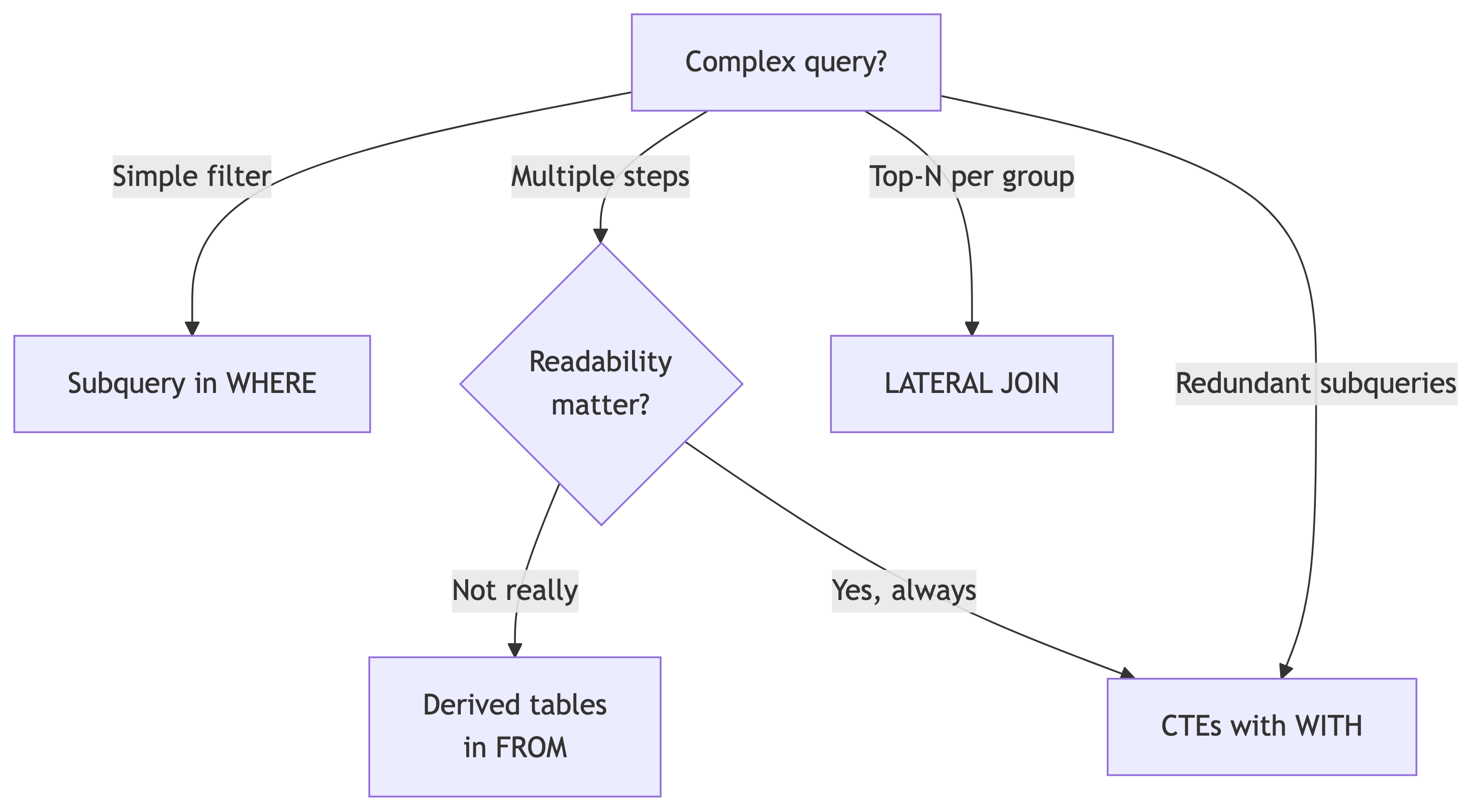
TL;DR;DS: When to Choose What

My honest take: CTEs > nested subqueries for readability. Always.

🧠 Quick Check: CTE Syntax

Which keyword starts a Common Table Expression?

A. CREATE TEMP TABLE
B. WITH
C. AS TABLE
D. DEFINE

B. The WITH keyword defines one or more CTEs. You can chain multiple CTEs separated by commas before the main SELECT. They’re sometimes called “WITH queries” for this reason.

Try It: State-Level Summary CTE 🎯

Using two CTEs, compute:

CTE 1: the total population per state
CTE 2: the number of counties per state

Join them and add a column for average population per county. Show state, total pop, county count, and avg pop per county. Order by average descending.

-- Your query here

WITH state_pop AS (
    SELECT state_name, sum(pop_est_2019) AS total_pop
    FROM us_counties_pop_est_2019
    GROUP BY state_name
),
state_counties AS (
    SELECT state_name, count(*) AS num_counties
    FROM us_counties_pop_est_2019
    GROUP BY state_name
)
SELECT sp.state_name,
       sp.total_pop,
       sc.num_counties,
       round(sp.total_pop::numeric / sc.num_counties, 0) AS avg_pop_per_county
FROM state_pop sp
JOIN state_counties sc ON sp.state_name = sc.state_name
ORDER BY avg_pop_per_county DESC;

Two clean, named steps, then a simple join. This is the CTE pattern at its best.

Part 6: Cross Tabulations

Pivot tables in SQL. Every analyst’s favorite party trick. 🎩

crosstab()

Enable the Extension

CREATE EXTENSION tablefunc;

This loads the crosstab() function from the tablefunc module. You only need to do this once per database. Standard ANSI SQL doesn’t have a crosstab function, but PostgreSQL provides one through its extension system.

The Ice Cream Survey

SELECT *
FROM ice_cream_survey
ORDER BY response_id
LIMIT 10;

200 employees across three offices, each picking a flavor. We want a pivot: offices as rows, flavors as columns, counts as values.

The raw data is “long format”: one row per response. We need “wide format”: one row per office with flavor counts as columns. That transformation is what crosstab() does.

Generating the Crosstab

SELECT *
FROM crosstab(
    'SELECT office, flavor, count(*)
     FROM ice_cream_survey
     GROUP BY office, flavor
     ORDER BY office',
    'SELECT flavor
     FROM ice_cream_survey
     GROUP BY flavor
     ORDER BY flavor'
)
AS (office text,
    chocolate bigint,
    strawberry bigint,
    vanilla bigint);

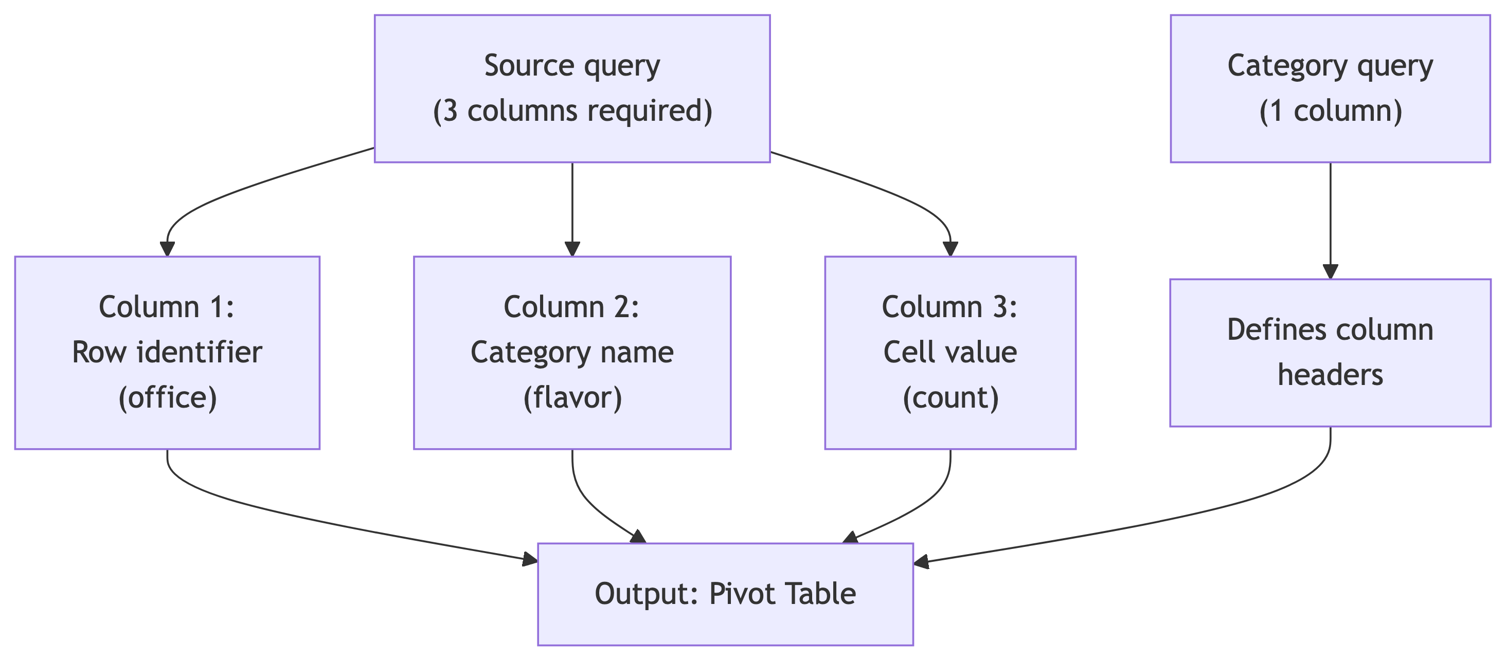
Run this. The first argument is the source query (must have exactly 3 columns: row name, category, value). The second argument defines the category labels. The AS clause names the output columns.

Takeaway: Midtown loves chocolate and has zero interest in strawberry (NULL). The Uptown office is more evenly split. Decisions made, ice cream ordered.

How crosstab() Works

Rules:

Source query: exactly 3 columns (row, category, value)
Category query: exactly 1 column (unique category values)
AS clause: must list output columns in the order the category query returns them
Both queries are passed as strings (single-quoted)
Escaped quotes inside: use '' (two single quotes)

Temperature Crosstab

A more complex example: median max temperature by station and month Run this. What are your observations?

SELECT *
FROM crosstab(
    'SELECT station_name,
            date_part(''month'', observation_date),
            percentile_cont(.5)
                WITHIN GROUP (ORDER BY max_temp)
     FROM temperature_readings
     GROUP BY station_name,
              date_part(''month'', observation_date)
     ORDER BY station_name',
    'SELECT month FROM generate_series(1,12) month'
)
AS (station text,
    jan numeric(3,0), feb numeric(3,0), mar numeric(3,0),
    apr numeric(3,0), may numeric(3,0), jun numeric(3,0),
    jul numeric(3,0), aug numeric(3,0), sep numeric(3,0),
    oct numeric(3,0), nov numeric(3,0), dec numeric(3,0));

Key Points on Previous Query

station	jan	feb	mar	apr	may	jun	jul	aug	sep	oct	nov	dec
CHICAGO NORTHERLY ISLAND IL US	34	36	46	50	66	77	81	80	77	65	57	35
SEATTLE BOEING FIELD WA US	50	54	56	64	66	71	76	77	69	62	55	42
WAIKIKI 717.2 HI US	83	84	84	86	87	87	88	87	87	86	84	82

Takeaway: Three stations, 12 months, median temperatures. generate_series(1,12) creates the month column headers. Waikiki is consistently balmy. Chicago goes from freezing to pleasant. Seattle splits the difference.

🧠 Quick Check: Crosstab Requirements

The source query for crosstab() must return exactly how many columns?

A. 2
B. 3
C. 4
D. It depends on the output

B. Always three: (1) row identifier, (2) category, (3) value. The row identifier groups the pivot rows, the category determines which output column gets the value. No more, no less.

Part 7: CASE Expressions

Conditional logic inside SQL. Your if/else for data transformation.

Reclassifying Values with CASE

The CASE Pattern

CASE
    WHEN condition THEN result
    WHEN another_condition THEN result
    ELSE fallback_result
END

Evaluates conditions top-to-bottom
Returns the first match and stops
ELSE catches anything that fell through
Without ELSE, unmatched rows get NULL
Works in SELECT, WHERE, ORDER BY, and aggregations

Think of it as a series of if/else-if/else blocks. Order matters: put your most specific conditions first.

Reclassifying Temperature Data

SELECT max_temp,
       CASE WHEN max_temp >= 90 THEN 'Hot'
            WHEN max_temp >= 70 AND max_temp < 90 THEN 'Warm'
            WHEN max_temp >= 50 AND max_temp < 70 THEN 'Pleasant'
            WHEN max_temp >= 33 AND max_temp < 50 THEN 'Cold'
            WHEN max_temp >= 20 AND max_temp < 33 THEN 'Frigid'
            WHEN max_temp < 20 THEN 'Inhumane'
            ELSE 'No reading'
       END AS temperature_group
FROM temperature_readings
ORDER BY station_name, observation_date;

Each row gets classified into a group. The ranges cover all possible values with no gaps. The ELSE clause is our safety net (and yes, “Inhumane” is an editorial choice, not a meteorological term).

May Dr. Gore grant me absolution. 🙌

CASE in a Common Table Expression (Steps)

Combine CASE with a CTE to classify, then aggregate. The two-step pattern:

Step 1 (CTE): classify every reading.
Step 2 (outer query): count days per station per group.

Temperatures Collapsed

Run this. What are your observations?

WITH temps_collapsed (station_name, max_temperature_group) AS (
    SELECT station_name,
           CASE WHEN max_temp >= 90 THEN 'Hot'
                WHEN max_temp >= 70 AND max_temp < 90 THEN 'Warm'
                WHEN max_temp >= 50 AND max_temp < 70 THEN 'Pleasant'
                WHEN max_temp >= 33 AND max_temp < 50 THEN 'Cold'
                WHEN max_temp >= 20 AND max_temp < 33 THEN 'Frigid'
                WHEN max_temp < 20 THEN 'Inhumane'
                ELSE 'No reading'
           END
    FROM temperature_readings
)
SELECT station_name, max_temperature_group, count(*)
FROM temps_collapsed
GROUP BY station_name, max_temperature_group
ORDER BY station_name, count(*) DESC;

Dataset Output from Previous Query

station_name	max_temperature_group	count
CHICAGO NORTHERLY ISLAND IL US	Warm	133
CHICAGO NORTHERLY ISLAND IL US	Cold	92
CHICAGO NORTHERLY ISLAND IL US	Pleasant	91
CHICAGO NORTHERLY ISLAND IL US	Frigid	30
CHICAGO NORTHERLY ISLAND IL US	Inhumane	8
CHICAGO NORTHERLY ISLAND IL US	Hot	8
SEATTLE BOEING FIELD WA US	Pleasant	198
SEATTLE BOEING FIELD WA US	Warm	98
SEATTLE BOEING FIELD WA US	Cold	50
SEATTLE BOEING FIELD WA US	Hot	3
WAIKIKI 717.2 HI US	Warm	361
WAIKIKI 717.2 HI US	Hot	5

My Takeaway

Waikiki has 361 Warm days. Chicago has 8 Inhumane days. I know where I’d rather be.

🏖️

🧠 Quick Check: CASE Evaluation

If a value of 95 is evaluated by a CASE statement where the first WHEN is max_temp >= 70 and the second is max_temp >= 90, what happens?

A. It matches the >= 90 condition
B. It matches the >= 70 condition (first match wins)
C. It matches both conditions
D. It returns NULL

B. CASE evaluates top-to-bottom and returns the first match. 95 >= 70 is true, so it returns that result and stops. It never checks >= 90. This is why you put the most restrictive conditions first (>= 90 before >= 70).

Try It: Population Tiers 🎯

Using a CTE with CASE on the us_counties_pop_est_2019 table, classify each county as:

‘Metro’ (pop >= 500,000)
‘Urban’ (pop 100,000 to 499,999)
‘Suburban’ (pop 50,000 to 99,999)
‘Rural’ (pop < 50,000)

Then count the number of counties in each tier and compute the total population per tier. Which tier has the most counties? Which holds the most population?

Columns: tier, num_counties, total_pop, avg_county_pop.

-- Your query here

Population Tiers Query

WITH county_tiers AS (
    SELECT county_name, state_name, pop_est_2019,
           CASE
               WHEN pop_est_2019 >= 500000 THEN 'Metro'
               WHEN pop_est_2019 >= 100000 THEN 'Urban'
               WHEN pop_est_2019 >= 50000 THEN 'Suburban'
               ELSE 'Rural'
           END AS tier
    FROM us_counties_pop_est_2019
)
SELECT tier,
       count(*) AS num_counties,
       sum(pop_est_2019) AS total_pop,
       round(avg(pop_est_2019), 0) AS avg_county_pop
FROM county_tiers
GROUP BY tier
ORDER BY total_pop DESC;

Takeaway: Rural has the most counties by far (~2,500+). Metro has the most total population. The vast majority of U.S. counties are small, but the vast majority of Americans live in big ones.

Part 8: Summary

What We Covered (a lot of ground! 🤯)

Key Techniques

Technique	What It Does	Textbook Listing
Scalar subquery in WHERE	Compute a threshold, filter on it	13-1
Subquery with DELETE	Filter rows to remove	13-2
Derived table (subquery in FROM)	Create a temporary table inline	13-3, 13-4
Column subquery in SELECT	Add a computed column per row	13-5, 13-6
`IN` with subquery	Check if value is in a result set	13-8
`EXISTS` / `NOT EXISTS`	Check membership (correlated)	13-9, 13-10
`LATERAL` in FROM	Reuse calculations across subqueries	13-11
`LATERAL` with JOIN	Per-row subquery (top-N per group)	13-12
CTE (`WITH`)	Named temporary result sets	13-13 to 13-15
`crosstab()`	Pivot long data to wide	13-17, 13-19
`CASE`	Conditional classification	13-20, 13-21

The Big Ideas

Subqueries go everywhere: WHERE, FROM, SELECT, even inside other subqueries and DML statements.
Know your correlation: Uncorrelated = runs once. Correlated = runs per row. The performance difference can be ginormous.
EXISTS short-circuits. For large-table membership checks, prefer it over IN. And never use NOT IN with nullable columns.
LATERAL is the top-N-per-group tool. “For each X, get the last N Y’s.” Learn it, love it.
CTEs > nested subqueries for readability. Always. Yes, I will die on this hill.
crosstab() = long to wide. Three columns in, pivot table out. Great for reporting.
CASE then aggregate. Classify first in a CTE, aggregate second in the outer query.

Up Next: In-Class Activity 🛠️

Time to practice! Open the Advanced Queries assignment in CodeGrade.

You’ll work through problems covering:

Scalar subqueries and derived tables
Correlated subqueries and EXISTS
LATERAL joins
CTEs
Cross tabulations and CASE

Use today’s lecture as your reference. You have ~30 minutes.

References

DeBarros, A. (2022). Practical SQL (2nd ed.). No Starch Press. Chapter 13.
PostgreSQL: WITH Queries (CTEs)
PostgreSQL: Subquery Expressions
PostgreSQL: LATERAL Joins
PostgreSQL: tablefunc (crosstab)