Lecture 13-1: Data Mining with Text

DATA 503: Fundamentals of Data Engineering

Lucas P. Cordova, Ph.D.

lpcordova@willamette.edu

Willamette University

April 6, 2026

What You’ll Learn

Learning Objectives

Apply common string functions for trimming, case conversion, measuring length, and slicing substrings
Read basic POSIX regex notation (\d, {n,m}, groups, alternation) and use ~, ~*, !~, and substring(... from ...)
Use regexp_match, regexp_matches, regexp_replace, and regexp_split_to_table to transform text
Extract structured columns from semi-structured blobs using capture groups and array indexing
Explain what tsvector and tsquery represent, use to_tsvector and to_tsquery (and when plainto_tsquery helps), and filter with @@ plus a GIN index
Use ts_headline for snippets and ts_rank for ordering matches (including length normalization)

Course Connection (where this fits)

Narrative text shows up in API responses, application logs, support exports, and “structured” CSVs that are mostly prose.
Regex plus full-text indexing are practical ways to normalize those fields near the database and to support search without assuming a dedicated search service.

Text is not a luxury column type. It is where half your “CSV from a government website” problems live. Today we give SQL something sharper than hope. 🙏

Part 1: Environment

Create the Database and Load Data

Create a dedicated database for this chapter using whatever method you prefer or the command above in a terminal.

createdb mining_text;

Load Data

Download and run the setup script mining_text.sql ↓ while connected to mining_text. The file embeds all rows with INSERT statements (dollar-quoted text), so you can run it from pgAdmin or Beekeeper without configuring server-side CSV paths.

You’re welcome. 😂

Optional: crime_reports.csv matches the embedded crime narratives if you want to practice client-side \copy from psql and compare it to the all-in-one script.

I won’t stop you! 😂

Tables You Will See Tonight 🌚

Table	Source	Role
`county_regex_demo`	bundled in `mining_text.sql`	Regex filtering practice (`~`, `~*`)
`crime_reports`	embedded in `mining_text.sql`	Parse semi-structured police narratives
`president_speeches`	embedded in `mining_text.sql`	Full-text search on State of the Union addresses

Sanity Checks 🛫

Run these after the setup script finishes to verify the counts of the tables.

SELECT count(*) FROM crime_reports;
-- 5
SELECT count(*) FROM president_speeches;
-- 79
SELECT count(*) FROM county_regex_demo;
-- 8

Part 2: String Functions

Why Strings Still Matter ❤️‍🔥

JSON gets the hype. Arrays get the conference talks. Strings pay the rent: addresses, notes, log lines, pasted emails, and whatever your stakeholder calls “structured” because it has a colon somewhere.

PostgreSQL’s string toolkit is documented in the manual under String Functions. We start with the ones you will actually type.

Casing and Cleanup

SELECT upper('Neal7');
SELECT lower('Randy');
SELECT initcap('at the end of the day');
SELECT initcap('Practical SQL');  -- acronyms: not perfect

Casing and Cleanup · Output

Run these in order and watch how forgiving real-world text is not.

SELECT upper('Neal7');
-- NEAL7
SELECT lower('Randy');
-- randy
SELECT initcap('at the end of the day');
-- At The End Of The Day
SELECT initcap('Practical SQL');  -- acronyms: not perfect
-- Practical Sql

initcap capitalizes word starts. It does not read minds. Your acronym table lives in application code, not here.

Length, Position, Trim

SELECT char_length(' Pat ');
SELECT length(' Pat ');          -- same for varchar; byte length differs on some types
SELECT position(', ' in 'Tan, Bella');
SELECT trim('s' from 'socks');
SELECT trim(trailing 's' from 'socks');
SELECT trim(' Pat ');
SELECT char_length(trim(' Pat '));
SELECT ltrim('socks', 's');
SELECT rtrim('socks', 's');

Length, Position, Trim · Output

Run these in order.

SELECT char_length(' Pat ');
-- 5
SELECT length(' Pat ');          -- same for varchar; byte length differs on some types
-- 5
SELECT position(', ' in 'Tan, Bella');
-- 4
SELECT trim('s' from 'socks');
-- ock
SELECT trim(trailing 's' from 'socks');
-- sock
SELECT trim(' Pat ');
-- Pat
SELECT char_length(trim(' Pat '));
-- 3
SELECT ltrim('socks', 's');
-- ocks
SELECT rtrim('socks', 's');
-- sock

If you are counting characters for validation rules, char_length after trim is the boring, correct path.

Slicing and Replacing

SELECT left('703-555-1212', 3);
SELECT right('703-555-1212', 8);
SELECT replace('bat', 'b', 'c');
SELECT replace('aaa', 'aa', 'b');

Slicing and Replacing · Output

Run these (including the replace('aaa', ...) check).

SELECT left('703-555-1212', 3);
-- 703
SELECT right('703-555-1212', 8);
-- 555-1212
SELECT replace('bat', 'b', 'c');
-- cat
SELECT replace('aaa', 'aa', 'b');
-- ba

Quick check: replace('aaa', 'aa', 'b') returns ba (left-to-right, non-overlapping substitution). String replacement is greedy in a way that will eventually humble everyone.

Part 3: Regular Expressions

What is a regular expression?

A regular expression (regex) is a small pattern language for describing text shape. You hand PostgreSQL a pattern string; the engine can test a match, return the matched substring, split on delimiters, or pull out captured pieces.

PostgreSQL uses POSIX regular expressions (documented under Pattern Matching). In SQL the pattern usually lives in a single-quoted string. Backslashes are easy to get wrong: the string parser and the regex engine both care about \, so you often write '\\d' (two characters in source, one backslash in the pattern) or use dollar-quoting when patterns get busy.

Notation

Piece	Meaning
`.`	one character (with caveats: not always newline)
`\d`	a digit `0`–`9`
`\w`	a word character (letters, digits, underscore in the POSIX class)
`[0-9]`	any single digit from the list
`{n}`	repeat the previous “atom” exactly `n` times
`{n,m}`	repeat at least `n` and at most `m` times, so `{1,2}` means one or two
`+`	one or more; `*` zero or more; `?` optional (zero or one)
`^` `$`	start and end of the string (for these lectures, think whole-field matching unless noted)
`\\|`	alternation: `A\\|B` is A or B
`()`	grouping; also capture for `regexp_match`
`(?: … )`	group without capturing (still useful for precedence)

Example

\d{1,2}/\d{1,2}/\d{2} describes a date fragment like 4/16/17: one or two digits, slash, one or two digits, slash, two digits. Slashes are literal here; we sometimes escape them as \/ in patterns for clarity or habit from other tools.

Operators Thou Shalt Know 🫠

Operator	Meaning
`~`	matches, case sensitive
`~*`	matches, case insensitive
`!~`	does not match, case sensitive
`!~*`	does not match, case insensitive

In WHERE clauses, regex turns a pile of LIKE patterns into one expressive filter. It also turns a simple bug into a performance mystery. Use indexes thoughtfully (later: GIN for FTS; for regex alone, sometimes a functional index, sometimes a redesign).

Substring with a Pattern

SELECT substring('The game starts at 7 p.m. on May 2, 2024.' from '.+');
SELECT substring('The game starts at 7 p.m. on May 2, 2024.' from '\d{1,2} (?:a.m.|p.m.)');
SELECT substring('The game starts at 7 p.m. on May 2, 2024.' from '^\w+');
SELECT substring('The game starts at 7 p.m. on May 2, 2024.' from '\w+.$');
SELECT substring('The game starts at 7 p.m. on May 2, 2024.' from 'May|June');
SELECT substring('The game starts at 7 p.m. on May 2, 2024.' from '\d{4}');
SELECT substring('The game starts at 7 p.m. on May 2, 2024.' from 'May \d, \d{4}');

Substring with a Pattern · Output

substring(string from pattern) returns the first match. Run them one at a time.

SELECT substring('The game starts at 7 p.m. on May 2, 2024.' from '.+');
-- The game starts at 7 p.m. on May 2, 2024.
SELECT substring('The game starts at 7 p.m. on May 2, 2024.' from '\d{1,2} (?:a.m.|p.m.)');
-- 7 p.m.
SELECT substring('The game starts at 7 p.m. on May 2, 2024.' from '^\w+');
-- The
SELECT substring('The game starts at 7 p.m. on May 2, 2024.' from '\w+.$');
-- 2024.
SELECT substring('The game starts at 7 p.m. on May 2, 2024.' from 'May|June');
-- May
SELECT substring('The game starts at 7 p.m. on May 2, 2024.' from '\d{4}');
-- 2024
SELECT substring('The game starts at 7 p.m. on May 2, 2024.' from 'May \d, \d{4}');
-- May 2, 2024

Notice how greedy .+ is on the first pattern. Regex is a contract between you and the parser. Read the contract. 🤝

Filtering Rows

We use county_regex_demo instead of the full Census extract.

Run a SELECT * FROM county_regex_demo; to see the data. What would these queries return?

SELECT county_name
FROM county_regex_demo
WHERE county_name ~* '(lade|lare)'
ORDER BY county_name;

SELECT county_name
FROM county_regex_demo
WHERE county_name ~* 'ash' AND county_name !~ 'Wash'
ORDER BY county_name;

Filtering Rows · Output

SELECT county_name
FROM county_regex_demo
WHERE county_name ~* '(lade|lare)'
ORDER BY county_name;
-- Clare County

SELECT county_name
FROM county_regex_demo
WHERE county_name ~* 'ash' AND county_name !~ 'Wash'
ORDER BY county_name;
-- Ashland County
-- Nash County

The second query is the classic “I want Ashland but not Washington” maneuver. If your data contains NULL county names, remember that WHERE col ~ 'pattern' does not match NULL.

Replacing and Splitting

Run these.

SELECT regexp_replace('05/12/2024', '\d{4}', '2023');
SELECT regexp_split_to_table('Four,score,and,seven,years,ago', ',');
SELECT regexp_split_to_array('Phil Mike Tony Steve', ' ');
SELECT array_length(regexp_split_to_array('Phil Mike Tony Steve', ' '), 1);

Replacing and Splitting · Output

SELECT regexp_replace('05/12/2024', '\d{4}', '2023');
-- 05/12/2023
SELECT regexp_split_to_table('Four,score,and,seven,years,ago', ',');
-- Four
-- score
-- and
-- seven
-- years
-- ago
SELECT regexp_split_to_array('Phil Mike Tony Steve', ' ');
-- {Phil,Mike,Tony,Steve}
SELECT array_length(regexp_split_to_array('Phil Mike Tony Steve', ' '), 1);
-- 4

regexp_split_to_table is a set-returning function: it produces one row per piece. That makes it handy for normalizing multi-valued cells.”

Part 4: From Blob to Columns

The Crime Narratives

Run a SELECT * FROM crime_reports; to see the data. What would this query return?

SELECT crime_id, original_text
FROM crime_reports
ORDER BY crime_id

The Crime Narratives · Output

Our crime_reports table loads only original_text. Everything else (dates, address, offense, case number) is hiding inside the blob.

Run this to open one row:

SELECT original_text
FROM crime_reports
ORDER BY crime_id
LIMIT 1;
-- 4/16/17-4/17/17
-- 2100-0900 hrs.
-- 46000 Block Ashmere Sq.
-- Sterling
-- Larceny: The victim reported that a
-- bicycle was stolen from their opened
-- garage door during the overnight hours.
-- C0170006614

Beautiful. Readable. Terrible for GROUP BY. We will fix that with patterns, not with interns.

First Date Match

Run this.

SELECT crime_id,
       regexp_match(original_text, '\d{1,2}\/\d{1,2}\/\d{2}')
FROM crime_reports
ORDER BY crime_id;

First Date Match · Output

regexp_match returns the first match as a text array (or NULL).

SELECT crime_id,
       regexp_match(original_text, '\d{1,2}\/\d{1,2}\/\d{2}')
FROM crime_reports
ORDER BY crime_id;
-- 1 | {4/16/17}
-- 2 | {4/8/17}
-- 3 | {4/4/17}
-- 4 | {04/10/17}
-- 5 | {04/09/17}

All Date Matches

Row 1 has two dates in the narrative.

4/16/17-4/17/17
2100-0900 hrs.
46000 Block Ashmere Sq.
Sterling

Run this and compare to the previous slide.

SELECT crime_id,
       regexp_matches(original_text, '\d{1,2}\/\d{1,2}\/\d{2}', 'g')
FROM crime_reports
ORDER BY crime_id;

All Date Matches · Output

regexp_matches with the g flag finds every non-overlapping match.

SELECT crime_id,
       regexp_matches(original_text, '\d{1,2}\/\d{1,2}\/\d{2}', 'g')
FROM crime_reports
ORDER BY crime_id;
-- 1 | {4/16/17}
-- 1 | {4/17/17}
-- 2 | {4/8/17}
-- 3 | {4/4/17}
-- 4 | {04/10/17}
-- 5 | {04/09/17}

Compare the two outputs for rows that mention more than one calendar date.

Capture Groups Clean Up Noise

Run these:

SELECT crime_id,
       regexp_match(original_text, '-\d{1,2}\/\d{1,2}\/\d{2}')
FROM crime_reports
ORDER BY crime_id;
SELECT crime_id,
       regexp_match(original_text, '-(\d{1,2}\/\d{1,2}\/\d{2})')
FROM crime_reports
ORDER BY crime_id;

Capture Groups · Output

Parentheses in the pattern define capture groups. regexp_match still returns the whole match as element [1] when you wrap only part of the pattern. Run both.

SELECT crime_id,
       regexp_match(original_text, '-\d{1,2}\/\d{1,2}\/\d{2}')
FROM crime_reports
ORDER BY crime_id;
-- 1 | {-4/17/17}
-- 2 |
-- 3 |
-- 4 |
-- 5 |
SELECT crime_id,
       regexp_match(original_text, '-(\d{1,2}\/\d{1,2}\/\d{2})')
FROM crime_reports
ORDER BY crime_id;
-- 1 | {4/17/17}
-- 2 |
-- 3 |
-- 4 |
-- 5 |

The second version drops the leading hyphen by capturing only the date digits.

Pull Several Fields at Once

Run this:

SELECT
    crime_id,
    regexp_match(original_text, '(?:C0|SO)[0-9]+') AS case_number,
    regexp_match(original_text, '\d{1,2}\/\d{1,2}\/\d{2}') AS date_1,
    regexp_match(original_text, '\n(?:\w+ \w+|\w+)\n(.*):') AS crime_type,
    regexp_match(original_text, '(?:Sq.|Plz.|Dr.|Ter.|Rd.)\n(\w+ \w+|\w+)\n')
        AS city
FROM crime_reports
ORDER BY crime_id;

Pull Several Fields · Output

This is not pretty, but it is honest.

SELECT
    crime_id,
    regexp_match(original_text, '(?:C0|SO)[0-9]+') AS case_number,
    regexp_match(original_text, '\d{1,2}\/\d{1,2}\/\d{2}') AS date_1,
    regexp_match(original_text, '\n(?:\w+ \w+|\w+)\n(.*):') AS crime_type,
    regexp_match(original_text, '(?:Sq.|Plz.|Dr.|Ter.|Rd.)\n(\w+ \w+|\w+)\n')
        AS city
FROM crime_reports
ORDER BY crime_id;
-- 1 | {C0170006614} | {4/16/17} | {Larceny} | {Sterling}
-- 2 | {C0170006162} | {4/8/17} | {Destruction of Property} | {Sterling}
-- 3 | {C0170006079} | {4/4/17} | {Larceny} | {Sterling}
-- 4 | {SO170006250} | {04/10/17} | {Larceny} | {Middleburg}
-- 5 | {SO170006211} | {04/09/17} | {Destruction of Property} | {Sterling}

Patterns like this are why we version-control SQL. The day the sheriff’s office changes a label from hrs. to hours, you will discover the true meaning of “breaking change.”

Arrays in PostgreSQL: `[1]`

Run this:

SELECT
    crime_id,
    (regexp_match(original_text, '(?:C0|SO)[0-9]+'))[1] AS case_number
FROM crime_reports
ORDER BY crime_id;

Arrays in PostgreSQL · Output

regexp_match returns text[]. Grab the first element explicitly.

SELECT
    crime_id,
    (regexp_match(original_text, '(?:C0|SO)[0-9]+'))[1] AS case_number
FROM crime_reports
ORDER BY crime_id;
-- 1 | C0170006614
-- 2 | C0170006162
-- 3 | C0170006079
-- 4 | SO170006250
-- 5 | SO170006211

If the match fails, regexp_match is NULL and [1] is NULL. Plan for that when you cast to timestamps.

Optional: Populate Columns

-- Pattern sketch (abbreviated): build a string, cast to timestamptz
-- ((regexp_match(...))[1] || ' ' || (regexp_match(...))[1])::timestamptz

Optional: Populate Columns · Notes

The textbook walks through UPDATE statements that cast extracted dates to timestamptz and fill street, city, crime_type, and description. The expressions are long but repetitive: once you trust one regexp_match, the rest are the same idea with different patterns.

Question for you: Why might EXISTS (SELECT regexp_matches(...)) appear in a CASE branch?

Answer

Because sometimes you need to know whether a second date exists before you try to parse it.

Walkthrough: Build `date_1` Once

⚠️Don’t run this (unless you are using a scratch database or copy of the crime_reports table):

CREATE temp TABLE crime_reports_copy AS SELECT * FROM crime_reports; -- ⬅︎ Do this first!

UPDATE crime_reports
SET date_1 =
(
    (regexp_match(original_text, '\d{1,2}\/\d{1,2}\/\d{2}'))[1]
        || ' ' ||
    (regexp_match(original_text, '\/\d{2}\n(\d{4})'))[1]
        || ' US/Eastern'
)::timestamptz
RETURNING crime_id, date_1, original_text; -- ⬅︎ WT is this?

Walkthrough: Build `date_1` · Output

The book examples concatenate dates with MM/DD/YY form with the first time field (four digits) and a time zone.

Run once (it updates every row). Use a scratch database or ROLLBACK if you are experimenting.

UPDATE crime_reports_copy -- ⬅︎ This is the copy... whew!
SET date_1 =
(
    (regexp_match(original_text, '\d{1,2}\/\d{1,2}\/\d{2}'))[1]
        || ' ' ||
    (regexp_match(original_text, '\/\d{2}\n(\d{4})'))[1]
        || ' US/Eastern'
)::timestamptz
RETURNING crime_id, date_1, original_text; -- ⬅︎ WT is this still?
-- 1 | 2017-04-17 01:00:00+00 | ...
-- 2 | 2017-04-08 20:00:00+00 | ...
-- 3 | 2017-04-04 18:00:00+00 | ...
-- 4 | 2017-04-10 20:05:00+00 | ...
-- 5 | 2017-04-09 16:00:00+00 | ...

Why `RETURNING`?

RETURNING shows you what you broke before you commit. This is not Tinder. Do not swipe right on untested regex.

If a row lacks one of the pieces, the corresponding regexp_match is NULL and the concatenation collapses in ways PostgreSQL will explain loudly. That is good. Silent failure is how you become a historian instead of a data engineer.

View the Cleaned Rows

Run this:

SELECT date_1,
       street,
       city,
       crime_type
FROM crime_reports_copy
ORDER BY crime_id;

View the Cleaned Rows · Output

After a full UPDATE of all parsed columns (as in the book), a simple report query becomes possible. The UPDATE sets date_1 only (other parsed columns stay NULL until you run the full UPDATE block that sets all parsed columns).

SELECT date_1,
       street,
       city,
       crime_type
FROM crime_reports_copy
ORDER BY crime_id;
-- 2017-04-17 01:00:00+00 |  |  | 
-- 2017-04-08 20:00:00+00 |  |  | 
-- 2017-04-04 18:00:00+00 |  |  | 
-- 2017-04-10 20:05:00+00 |  |  | 
-- 2017-04-09 16:00:00+00 |  |  |

Compare mentally to the blob you started with. That difference is the whole lecture in one SELECT.

Part 5: Full-Text Search

Pipeline: From Speech to Search

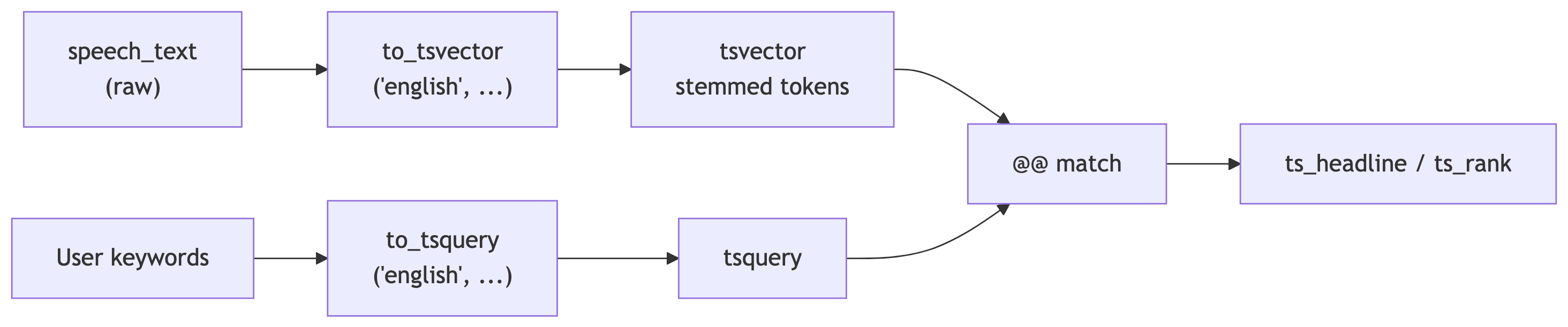
Raw text becomes a tsvector via to_tsvector. User or application text becomes a tsquery via to_tsquery (or helpers such as plainto_tsquery). The @@ operator tests whether a document matches a query. ts_headline and ts_rank sit after that: snippets and sort order for the matching rows. The GIN index sits on the stored tsvector so @@ does not devolve into a sequential scan over every speech.

`pg_ts_config`

Run this:

SELECT cfgname FROM pg_ts_config;

`pg_ts_config` · Output

Full-text search is not LIKE '%tax%'. It tokenizes, stems, drops noise words, and gives you operators that behave well at scale.

Check which language configurations exist.

SELECT cfgname FROM pg_ts_config;
-- arabic
-- armenian
-- basque
-- catalan
-- danish
-- dutch
-- english
-- finnish
-- ... (more rows on your server)

Documents vs queries: `tsvector` and `tsquery`

PostgreSQL full-text search works with two structured types, not raw text alone.

A tsvector is the document side: a normalized list of lexemes (stemmed tokens), usually with positions (and optional weights). It answers “what searchable terms does this row contain, and where?”
A tsquery is the query side: lexemes plus boolean and proximity operators. It answers “what pattern of terms are we looking for?”

You convert text into each form with functions (to_tsvector, to_tsquery, and related helpers). The match operator @@ compares a tsvector to a tsquery and returns true or false.

`to_tsvector`: from prose to a searchable document

to_tsvector('english', some_text) (first argument is a text search configuration name or regconfig) does the linguistic work on the document:

Tokenize into words
Drop stop words (common words the config treats as noise, often the, am, and similar)
Normalize and stem so related forms line up (for example walking and walk can converge to the same lexeme)

What it is for: producing the indexed, comparable form of a blob of text. In pipelines you often store a tsvector column (here search_speech_text) so you are not re-tokenizing on every search, and so a GIN index can target stable values.

Building a `tsquery`: `to_tsquery` and related functions

You need a tsquery on the right-hand side of @@. Common builders:

Function	Role
`to_tsquery(config, string)`	Parses a search string you write. You insert operators yourself (`&`, `\|`, `!`, `<->`, `<N>`). Powerful; best when your code builds the string.
`plainto_tsquery(config, string)`	Turns plain language into an AND of terms (after normalization). Handy for simple user-typed keywords without special syntax.
`phraseto_tsquery(config, string)`	Treats the string as a phrase (adjacent terms after tokenization).

This lecture uses to_tsquery so you see operators explicitly. In an app you might combine plainto_tsquery or validated user input with server-side templates.

`@@`: the match predicate

tsvector @@ tsquery returns boolean.

What it is for: the WHERE clause (and index conditions) that decides which rows participate in search. Everything else (ts_headline, ts_rank) is presentation or ordering on rows that already passed @@ (or on expressions you know match).

Typical pattern: WHERE search_speech_text @@ to_tsquery('english', 'vietnam').

Try it: `to_tsvector`, `to_tsquery`, and `@@`

SELECT to_tsvector('english', 'I am walking across the sitting room to sit with you.');

SELECT to_tsquery('english', 'walking & sitting');

SELECT to_tsvector('english', 'I am walking across the sitting room')
       @@ to_tsquery('english', 'walking & sitting');

SELECT to_tsvector('english', 'I am walking across the sitting room')
       @@ to_tsquery('english', 'walking & running');

Try it: output

Run these to see the stemmed lexemes, the parsed query, and the boolean match.

SELECT to_tsvector('english', 'I am walking across the sitting room to sit with you.');
-- 'across':4 'room':7 'sit':6,9 'walk':3

SELECT to_tsquery('english', 'walking & sitting');
-- 'walk' & 'sit'

SELECT to_tsvector('english', 'I am walking across the sitting room')
       @@ to_tsquery('english', 'walking & sitting');
-- t

SELECT to_tsvector('english', 'I am walking across the sitting room')
       @@ to_tsquery('english', 'walking & running');
-- f

Notice the document and query both pass through the same english config so stems line up (walking becomes walk in both worlds).

Operators Inside `to_tsquery`

& AND
| OR
! NOT
<-> adjacent terms (phrase)
<N> distance (terms within N positions)

We will lean on the State of the Union table. The setup script adds a tsvector column named search_speech_text. The next slides explain the GIN index that makes @@ queries scale.

What is GIN?

GIN stands for Generalized Inverted Index.

An inverted index flips the problem: instead of “for each row, what words does it have?” it stores “for each lexeme (stemmed token), which rows point at it?” That is exactly what @@ needs when it asks whether a document tsvector matches a tsquery.

Each indexed value is a tsvector: a list of lexemes with optional position and weight data. PostgreSQL walks the query tokens, looks them up in the inverted structure, and intersects or combines posting lists to find candidate rows.

Why GIN on `tsvector`, not a B-tree on `text`?

A B-tree is great for equality, range order, and prefix scans on a scalar column. It does not give you fast “contains these stemmed tokens anywhere in the document” semantics.

Full-text search matches on the precomputed tsvector column (search_speech_text), not on raw speech_text. You keep raw text for display; you match and rank on the vector. The GIN index is built on that vector column.

For tsvector, GIN is the usual default. GiST is an alternative with different update and recall trade-offs; for typical read-heavy search, GIN is the common choice.

GIN: read vs write trade-offs

Reads: Index-supported WHERE search_speech_text @@ to_tsquery(...) can use a bitmap index scan instead of reading every speech. That is the win you want in production.

Writes: Inserts and updates must maintain the inverted lists, so indexed columns cost more than an unindexed text column. Big bulk loads often finish the data, then build the index (or defer index creation until after load).

If you skip the index, search still returns correct results. The database just does a sequential scan and evaluates @@ per row. Fine for tiny tables; painful at scale.

Creating the GIN index

-- Already in mining_text.sql after INSERT + UPDATE:
-- CREATE INDEX search_idx ON president_speeches USING gin (search_speech_text);

USING gin tells PostgreSQL which access method to use. The indexed expression is the tsvector column, not a function of raw text (you already materialized the vector in search_speech_text).

Checking that the planner uses the index

After the index exists, a search like the next slide should show an index scan or bitmap index scan on search_idx in EXPLAIN (ANALYZE, BUFFERS) on a large enough table. If you see Seq Scan on president_speeches with only a handful of rows, the planner may still choose a sequential read, and that can be rational.

Without any GIN index on tsvector, expect sequential scans for @@ filters as the table grows.

Find Speeches

Run this:

SELECT president, speech_date
FROM president_speeches
WHERE search_speech_text @@ to_tsquery('english', 'Vietnam')
ORDER BY speech_date;

Find Speeches · Output

SELECT president, speech_date
FROM president_speeches
WHERE search_speech_text @@ to_tsquery('english', 'Vietnam')
ORDER BY speech_date;
-- John F. Kennedy | 1961-05-25
-- Lyndon B. Johnson | 1966-01-12
-- Lyndon B. Johnson | 1967-01-10
-- ... (16 more rows; 19 total in this bundle)

`ts_headline`: what it does and when to use it

Inputs: a text column to display (usually the original speech_text), a tsquery that describes the hit, and optional formatting options (how many words around the hit, delimiter strings for highlights).

What it does: picks a short excerpt that contains a good match and marks the matching terms (here with < and > around hits). It does not decide whether the row matches; use @@ in WHERE for that.

What it is for: search UIs (result snippets), email-style previews, and anywhere users need context without loading the full document. You still filter with search_speech_text @@ ... first; ts_headline is presentation layer on top.

Snippets with ts_headline

Run this:

SELECT president,
       speech_date,
       ts_headline(
           speech_text,
           to_tsquery('english', 'tax'),
           'StartSel = <,
            StopSel = >,
            MinWords=5,
            MaxWords=7,
            MaxFragments=1'
       )
FROM president_speeches
WHERE search_speech_text @@ to_tsquery('english', 'tax')
ORDER BY speech_date;

Snippets with ts_headline · Output

SELECT president,
       speech_date,
       ts_headline(
           speech_text,
           to_tsquery('english', 'tax'),
           'StartSel = <,
            StopSel = >,
            MinWords=5,
            MaxWords=7,
            MaxFragments=1'
       )
FROM president_speeches
WHERE search_speech_text @@ to_tsquery('english', 'tax')
ORDER BY speech_date;
-- Harry S. Truman | 1946-01-21 | ... <tax> POLICY ...
-- Harry S. Truman | 1947-01-06 | excise <tax> rates which, under the present
-- Harry S. Truman | 1948-01-07 | point in our <tax> structure. ...
-- ... (many more rows mention tax)

That angle-bracket markup is for HTML consumers. In slides, it still reads clearly as “here is the hit in context.”

AND / NOT and Phrase Proximity

Run each query:

SELECT president,
       speech_date,
       ts_headline(
           speech_text,
           to_tsquery('english', 'transportation & !roads'),
           'StartSel = <, StopSel = >, MinWords=5, MaxWords=7, MaxFragments=1'
       )
FROM president_speeches
WHERE search_speech_text @@ to_tsquery('english', 'transportation & !roads')
ORDER BY speech_date;
SELECT president,
       speech_date,
       ts_headline(
           speech_text,
           to_tsquery('english', 'military <-> defense'),
           'StartSel = <, StopSel = >, MinWords=5, MaxWords=7, MaxFragments=1'
       )
FROM president_speeches
WHERE search_speech_text @@ to_tsquery('english', 'military <-> defense')
ORDER BY speech_date;

AND / NOT and Phrase Proximity · Output

SELECT president,
       speech_date,
       ts_headline(
           speech_text,
           to_tsquery('english', 'transportation & !roads'),
           'StartSel = <, StopSel = >, MinWords=5, MaxWords=7, MaxFragments=1'
       )
FROM president_speeches
WHERE search_speech_text @@ to_tsquery('english', 'transportation & !roads')
ORDER BY speech_date;
-- Harry S. Truman | 1947-01-06 | Mr. President, Mr. Speaker, Members
-- Harry S. Truman | 1949-01-05 | Mr. President, Mr. Speaker, Members
SELECT president,
       speech_date,
       ts_headline(
           speech_text,
           to_tsquery('english', 'military <-> defense'),
           'StartSel = <, StopSel = >, MinWords=5, MaxWords=7, MaxFragments=1'
       )
FROM president_speeches
WHERE search_speech_text @@ to_tsquery('english', 'military <-> defense')
ORDER BY speech_date;
-- Dwight D. Eisenhower | 1956-01-05 | To the Congress of the
-- Dwight D. Eisenhower | 1958-01-09 | Mr. President, Mr. Speaker, Members
-- Dwight D. Eisenhower | 1959-01-09 | Mr. President, Mr. Speaker, Members

Try <2> instead of <-> in a copy of the query to allow a small gap between words. Language is messy. PostgreSQL knows.

`ts_rank`: what it does and when to use it

Inputs: a tsvector (the indexed document form) and a tsquery.

What it does: assigns a numeric relevance score based on how often query terms appear in the document vector (and related weighting). Higher scores mean “more query overlap” in a loose sense.

What it is for: sorting result sets when many rows satisfy @@. It is not a calibrated probability or a user-facing “percent match”; treat it as a relative ordering signal within one query.

Optional normalization: ts_rank(vector, query, 2) uses a normalization mode that penalizes long documents so a twenty-page speech does not always outrank a short one just because it repeats words more often. Compare ordering with and without that flag on the next slide.

Ranking

Run both and compare ordering.

SELECT president,
       speech_date,
       ts_rank(
           search_speech_text,
           to_tsquery('english', 'war & security & threat & enemy')
       ) AS score
FROM president_speeches
WHERE search_speech_text @@
      to_tsquery('english', 'war & security & threat & enemy')
ORDER BY score DESC
LIMIT 5;
SELECT president,
       speech_date,
       ts_rank(
           search_speech_text,
           to_tsquery('english', 'war & security & threat & enemy'),
           2
       )::numeric AS score
FROM president_speeches
WHERE search_speech_text @@
      to_tsquery('english', 'war & security & threat & enemy')
ORDER BY score DESC
LIMIT 5;

Ranking · Output

SELECT president,
       speech_date,
       ts_rank(
           search_speech_text,
           to_tsquery('english', 'war & security & threat & enemy')
       ) AS score
FROM president_speeches
WHERE search_speech_text @@
      to_tsquery('english', 'war & security & threat & enemy')
ORDER BY score DESC
LIMIT 5;
-- William J. Clinton | 1997-02-04 | 0.35810584
-- George W. Bush | 2004-01-20 | 0.29587495
-- George W. Bush | 2003-01-28 | 0.28381455
-- Harry S. Truman | 1946-01-21 | 0.25752166
-- William J. Clinton | 2000-01-27 | 0.22214262
SELECT president,
       speech_date,
       ts_rank(
           search_speech_text,
           to_tsquery('english', 'war & security & threat & enemy'),
           2
       )::numeric AS score
FROM president_speeches
WHERE search_speech_text @@
      to_tsquery('english', 'war & security & threat & enemy')
ORDER BY score DESC
LIMIT 5;
-- George W. Bush | 2004-01-20 | 0.000103
-- William J. Clinton | 1997-02-04 | 0.000098
-- George W. Bush | 2003-01-28 | 0.000096
-- Jimmy Carter | 1979-01-23 | 0.000090
-- Lyndon B. Johnson | 1968-01-17 | 0.000073

Long speeches accumulate token hits. Normalization option 2 divides rank by document length.

Compare the ordering before and after normalization. This is the difference between “mentions the keywords a lot” and “mentions them a lot relative to length.”

The book points to a live demo at anthonydebarros.com/sotu. Worth clicking after class.

Part 6: Practice and Pitfalls

Try It: Crime Case Numbers

Write a query that returns crime_id and the case number extracted from original_text using the same (?:C0|SO)[0-9]+ pattern, but filter to rows where the case starts with SO.

Stretch: Add a column that counts how many distinct dates appear in the narrative using regexp_matches with the g flag and a subquery or lateral trick. (If you get stuck, move on. The point is to think in matches, not to win a Nobel prize in SQL golf.)

Try It: Speeches

Find speeches where the query economy & jobs matches, show ts_headline, and sort by normalized rank (ts_rank with the length divisor). Pick a president you have opinions about. Keep the opinions out of the query.

Common Footguns (Collected)

Forgetting that regexp_match returns NULL when nothing matches, then indexing [1] in a cast chain
Using LIKE patterns with regex operators by mistake (they are not interchangeable)
Building huge OR chains when a single well-factored regex would do
Skipping the GIN index on tsvector columns and wondering why search “works on my laptop”

Summary

What We Covered

Topic	Core functions and ideas
Strings	`upper`, `lower`, `initcap`, `trim`, `left`/`right`, `replace`, `char_length`
Regex filters	`~`, `~*`, `!~`, `substring`, `regexp_replace`, splits
Structured extraction	`regexp_match`, `regexp_matches`, capture groups, `[1]` indexing
Full-text search	`tsvector` / `tsquery` types; `to_tsvector`, `to_tsquery`, `plainto_tsquery`; `@@`; `ts_headline`, `ts_rank`
Performance	GIN (inverted index on `tsvector`); favors search reads over cheap writes

The One-Sentence Version

Treat text like data: measure it, constrain it, extract what you need, and index what you search. Everything else is a spreadsheet someone emailed you as prose.

References

DeBarros, A. (2022). Practical SQL (2nd ed.). No Starch Press. Chapter 14.
PostgreSQL: Pattern Matching
PostgreSQL: String Functions
PostgreSQL: Regular Expressions
PostgreSQL: Full Text Search
PostgreSQL: ts_rank

Lecture 13-1: Data Mining with Text

What You’ll Learn

Learning Objectives

Course Connection (where this fits)

Part 1: Environment

Create the Database and Load Data

Load Data

Tables You Will See Tonight 🌚

Sanity Checks 🛫

Part 2: String Functions

Why Strings Still Matter ❤️‍🔥

Casing and Cleanup

Casing and Cleanup · Output

Length, Position, Trim

Length, Position, Trim · Output

Slicing and Replacing

Slicing and Replacing · Output

Part 3: Regular Expressions

What is a regular expression?

Notation

Example

Operators Thou Shalt Know 🫠

Substring with a Pattern

Substring with a Pattern · Output

Filtering Rows

Filtering Rows · Output

Replacing and Splitting

Replacing and Splitting · Output

Part 4: From Blob to Columns

The Crime Narratives

The Crime Narratives · Output

First Date Match

First Date Match · Output

All Date Matches

All Date Matches · Output

Capture Groups Clean Up Noise

Capture Groups · Output

Pull Several Fields at Once

Pull Several Fields · Output

Arrays in PostgreSQL: [1]

Arrays in PostgreSQL · Output

Optional: Populate Columns

Optional: Populate Columns · Notes

Answer

Walkthrough: Build date_1 Once

Walkthrough: Build date_1 · Output

Why RETURNING?

View the Cleaned Rows

View the Cleaned Rows · Output

Part 5: Full-Text Search

Pipeline: From Speech to Search

pg_ts_config

pg_ts_config · Output

Documents vs queries: tsvector and tsquery

to_tsvector: from prose to a searchable document

Building a tsquery: to_tsquery and related functions

@@: the match predicate

Try it: to_tsvector, to_tsquery, and @@

Try it: output

Operators Inside to_tsquery

What is GIN?

Why GIN on tsvector, not a B-tree on text?

GIN: read vs write trade-offs

Creating the GIN index

Checking that the planner uses the index

Find Speeches

Find Speeches · Output

ts_headline: what it does and when to use it

Snippets with ts_headline

Snippets with ts_headline · Output

AND / NOT and Phrase Proximity

AND / NOT and Phrase Proximity · Output

ts_rank: what it does and when to use it

Ranking

Ranking · Output

Part 6: Practice and Pitfalls

Try It: Crime Case Numbers

Try It: Speeches

Common Footguns (Collected)

Summary

Arrays in PostgreSQL: `[1]`

Walkthrough: Build `date_1` Once

Walkthrough: Build `date_1` · Output

Why `RETURNING`?

`pg_ts_config`

`pg_ts_config` · Output

Documents vs queries: `tsvector` and `tsquery`

`to_tsvector`: from prose to a searchable document

Building a `tsquery`: `to_tsquery` and related functions

`@@`: the match predicate

Try it: `to_tsvector`, `to_tsquery`, and `@@`

Operators Inside `to_tsquery`

Why GIN on `tsvector`, not a B-tree on `text`?

`ts_headline`: what it does and when to use it

`ts_rank`: what it does and when to use it