Dashboards with Grafana

DATA 503: Fundamentals of Data Engineering

Lucas P. Cordova, Ph.D.

lpcordova@willamette.edu

Willamette University

April 6, 2026

Learning Objectives

What You Will Be Able to Do

Explain where dashboards sit in a pipeline and why Grafana is a reasonable choice for SQL-backed analytics
Read and reason about dashboard-oriented views (aggregations, joins, classifications)
Interpret crosstab() pivots from tablefunc and know when a table panel in Grafana is the right visualization
Provision PostgreSQL 18 on Railway and restore a custom-format dump with pg_restore using the public database URL
Deploy Grafana on Railway with a separate grafana database for persistence and connect it to pipeline data with a read-only role
Build several panel types (bar, horizontal bar, grouped bar, table) from named views and pivot queries

Course Connection

This ties ingestion and modeling work to stakeholder-facing delivery: live, shareable visuals over the same database your pipeline maintains.

Part 1: Dashboards in the Pipeline

The Presentation Layer

Dashboards are the presentation layer. They turn vetted SQL into charts and tables other people can read without learning JOIN syntax.

Where Grafana Sits

Grafana does not replace your ETL jobs. It reads from PostgreSQL (ideally through views and restricted users) and renders results on a schedule or on demand.

What Makes a Good Pipeline Dashboard?

Live connection to the database, not a one-off CSV export
Refresh so panels stay current as data lands
Shareable links for reviews and demos
Layered layout: headline metrics on top, comparisons in the middle, detail tables below

Part 2: Grafana Overview

What Grafana Is

Grafana is an open-source observability and dashboarding platform. It started in metrics and logs, but its PostgreSQL data source is mature: you write SQL, Grafana maps columns to charts.

Why Grafana for This Course?

PostgreSQL-native data source with a SQL editor
Many panel types: time series, bar, table, stat, pie, heatmap, and more
Variables for filters (dropdowns that rewrite queries)
Alerting when a query crosses a threshold
Fits Railway: can run next to your database; serverless mode reduces idle cost

Grafana Architecture (Two Databases)

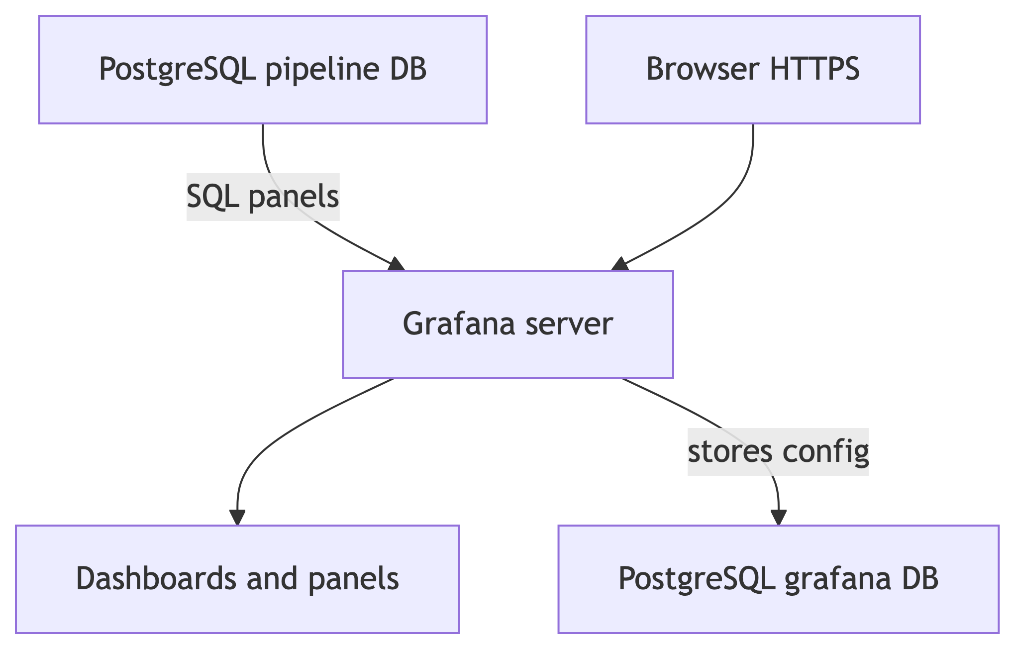
Analytics data lives in your pipeline database (after restore, that is the class dataset).
Grafana metadata (dashboards, users, data source definitions) should live in a separate database so you can rebuild or clone pipeline data without losing UI work.

Part 3: Views for Dashboards

Why Views?

A view is a named SELECT. It behaves like a read-only table for clients.

Hides long joins and aggregations behind one name
Reuse the same logic from Grafana, APIs, and ad hoc queries
Lets you grant SELECT on views to a read-only role without exposing base tables
When logic changes, you update the view once, not every panel

Views do not magically cache results unless you use a materialized view. For class-scale data, ordinary views are fine.

Dataset After Restore

After you restore railway_dump.dump, you should see the census, business, temperature, and survey tables from the advanced-queries style curriculum, plus the views below (names may match exactly).

Table	Approximate role
`us_counties_pop_est_2019`	County population and components of change
`cbp_naics_72_establishments`	Food and accommodation establishments by area
`temperature_readings`	Daily readings for three stations
`ice_cream_survey`	Long-format survey responses

Part 4: Dashboard-Ready Views (Review)

View: `v_state_population_summary`

State-level totals and natural increase. Good for sorted bar charts or tables.

CREATE OR REPLACE VIEW v_state_population_summary AS
SELECT
    state_name,
    count(*) AS num_counties,
    sum(pop_est_2019) AS total_pop,
    round(avg(pop_est_2019), 0) AS avg_county_pop,
    sum(births_2019) AS total_births,
    sum(deaths_2019) AS total_deaths,
    sum(births_2019) - sum(deaths_2019) AS natural_increase
FROM us_counties_pop_est_2019
GROUP BY state_name
ORDER BY total_pop DESC;

View: `v_state_migration_rates`

Rates per thousand and a direction label. Good for horizontal bar charts and color by category.

CREATE OR REPLACE VIEW v_state_migration_rates AS
WITH state_migration AS (
    SELECT
        state_name,
        sum(international_migr_2019 + domestic_migr_2019) AS net_migration,
        sum(pop_est_2018) AS base_pop
    FROM us_counties_pop_est_2019
    GROUP BY state_name
)
SELECT
    state_name,
    base_pop,
    net_migration,
    round((net_migration / base_pop::numeric) * 1000, 2) AS migration_rate_per_thousand,
    CASE
        WHEN net_migration > 0 THEN 'Gaining'
        WHEN net_migration < 0 THEN 'Losing'
        ELSE 'Stable'
    END AS migration_direction
FROM state_migration
ORDER BY migration_rate_per_thousand DESC;

View: `v_county_growth_summary`

Aggregates counties by growth category. Natural pie or stat panels.

CREATE OR REPLACE VIEW v_county_growth_summary AS
WITH county_growth AS (
    SELECT
        county_name,
        state_name,
        pop_est_2019,
        CASE
            WHEN pop_est_2019 > pop_est_2018 THEN 'Growing'
            WHEN pop_est_2019 < pop_est_2018 THEN 'Shrinking'
            ELSE 'Stable'
        END AS growth_category
    FROM us_counties_pop_est_2019
)
SELECT
    growth_category,
    count(*) AS num_counties,
    sum(pop_est_2019) AS total_pop,
    round(avg(pop_est_2019), 0) AS avg_county_pop,
    round(count(*)::numeric / (SELECT count(*) FROM us_counties_pop_est_2019) * 100, 1)
        AS pct_of_counties
FROM county_growth
GROUP BY growth_category
ORDER BY num_counties DESC;

View: `v_state_estabs_per_capita`

Establishments per thousand residents by state. Good ranked bar chart.

CREATE OR REPLACE VIEW v_state_estabs_per_capita AS
WITH estabs AS (
    SELECT st, sum(establishments) AS establishment_count
    FROM cbp_naics_72_establishments
    GROUP BY st
),
pop AS (
    SELECT state_name, sum(pop_est_2018) AS total_pop
    FROM us_counties_pop_est_2019
    GROUP BY state_name
)
SELECT
    pop.state_name,
    pop.total_pop,
    estabs.establishment_count,
    round((estabs.establishment_count / pop.total_pop::numeric) * 1000, 1)
        AS estabs_per_thousand
FROM estabs
JOIN pop ON estabs.st = pop.state_name
ORDER BY estabs_per_thousand DESC;

View: `v_seasonal_temperatures`

Season labels for each station. Ideal grouped bar chart.

CREATE OR REPLACE VIEW v_seasonal_temperatures AS
WITH labeled_readings AS (
    SELECT
        station_name,
        CASE
            WHEN date_part('month', observation_date) IN (12, 1, 2) THEN 'Winter'
            WHEN date_part('month', observation_date) IN (3, 4, 5)  THEN 'Spring'
            WHEN date_part('month', observation_date) IN (6, 7, 8)  THEN 'Summer'
            WHEN date_part('month', observation_date) IN (9, 10, 11) THEN 'Fall'
        END AS season,
        max_temp,
        min_temp
    FROM temperature_readings
)
SELECT
    station_name,
    season,
    round(avg(max_temp), 1) AS avg_max_temp,
    round(avg(min_temp), 1) AS avg_min_temp,
    count(*) AS num_readings
FROM labeled_readings
GROUP BY station_name, season
ORDER BY station_name,
    CASE season
        WHEN 'Winter' THEN 1
        WHEN 'Spring' THEN 2
        WHEN 'Summer' THEN 3
        WHEN 'Fall' THEN 4
    END;

View: `v_population_tiers`

County tiers by size. Strong population share story in one table.

CREATE OR REPLACE VIEW v_population_tiers AS
WITH tiers AS (
    SELECT
        county_name,
        state_name,
        pop_est_2019,
        CASE
            WHEN pop_est_2019 >= 500000 THEN 'Metro'
            WHEN pop_est_2019 >= 100000 THEN 'Urban'
            WHEN pop_est_2019 >= 50000 THEN 'Suburban'
            ELSE 'Rural'
        END AS tier
    FROM us_counties_pop_est_2019
)
SELECT
    tier,
    count(*) AS num_counties,
    sum(pop_est_2019) AS total_pop,
    round(avg(pop_est_2019), 0) AS avg_county_pop,
    round(sum(pop_est_2019)::numeric /
        (SELECT sum(pop_est_2019) FROM us_counties_pop_est_2019) * 100, 1)
        AS pct_of_total_pop
FROM tiers
GROUP BY tier
ORDER BY
    CASE tier
        WHEN 'Metro' THEN 1
        WHEN 'Urban' THEN 2
        WHEN 'Suburban' THEN 3
        WHEN 'Rural' THEN 4
    END;

Quick Check: Views vs. Inline SQL in Grafana

Why define views instead of pasting huge queries into every panel?

A. Views always cache results for Grafana
B. Views give a stable, reusable interface and cleaner permissions
C. Grafana cannot run SQL
D. Views refresh on a timer automatically

B. Non-materialized views still run fresh SQL. The win is naming, reuse, and security boundaries.

Part 5: Crosstabs and Pivot-Style Reporting

`tablefunc` and Long-to-Wide Data

Reporting often needs wide tables: one row per entity, many metric columns. Raw surveys and events are usually long: one row per observation.

PostgreSQL provides crosstab() through the extension:

CREATE EXTENSION IF NOT EXISTS tablefunc;

Ice Cream Survey Pivot

Long format: one row per person and flavor choice. Wide format: offices on rows, flavors as columns.

SELECT *
FROM crosstab(
    'SELECT office, flavor, count(*)
     FROM ice_cream_survey
     GROUP BY office, flavor
     ORDER BY office',
    'SELECT flavor
     FROM ice_cream_survey
     GROUP BY flavor
     ORDER BY flavor'
)
AS (office text,
    chocolate bigint,
    strawberry bigint,
    vanilla bigint);

Grafana note: This returns a table shape. Use a Table panel, not a bar chart, unless you unpivot again in SQL.

Temperature Median Pivot by Month

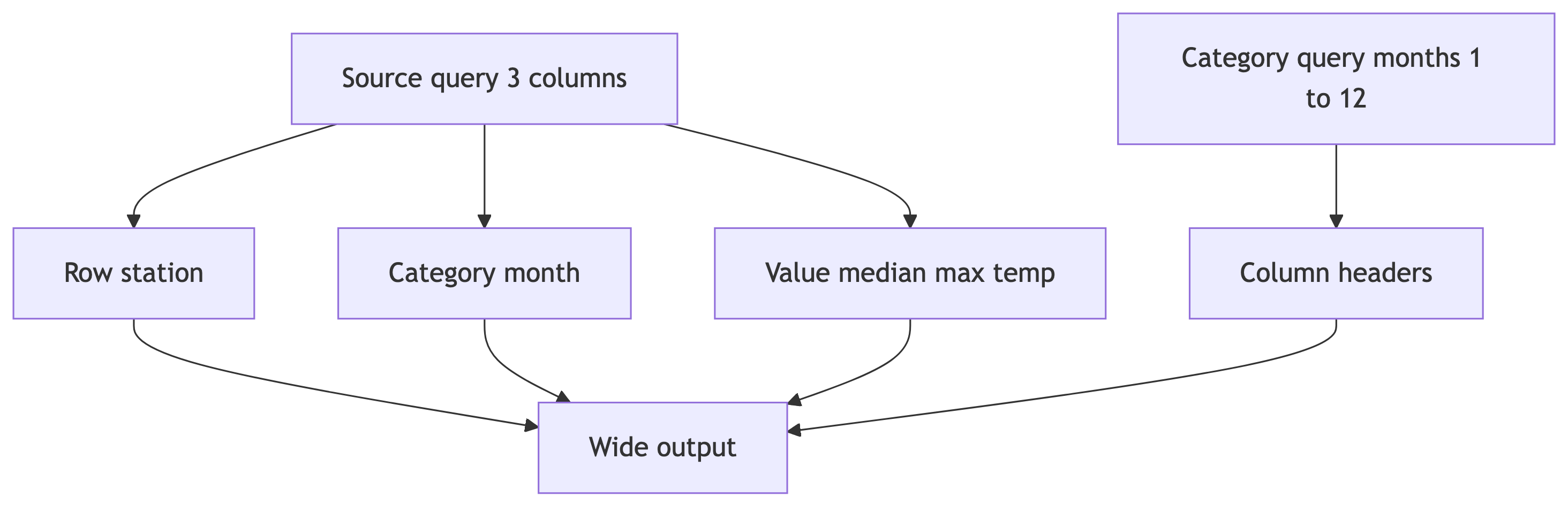
SELECT *
FROM crosstab(
    'SELECT station_name,
            date_part(''month'', observation_date),
            percentile_cont(.5)
                WITHIN GROUP (ORDER BY max_temp)
     FROM temperature_readings
     GROUP BY station_name,
              date_part(''month'', observation_date)
     ORDER BY station_name',
    'SELECT month FROM generate_series(1,12) month'
)
AS (station text,
    jan numeric(3,0), feb numeric(3,0), mar numeric(3,0),
    apr numeric(3,0), may numeric(3,0), jun numeric(3,0),
    jul numeric(3,0), aug numeric(3,0), sep numeric(3,0),
    oct numeric(3,0), nov numeric(3,0), dec numeric(3,0));

Quick Check: `crosstab()` Shape

The source query passed to crosstab() must return how many columns?

A. 2
B. 3
C. 4
D. It depends on the number of categories

B. Row id, category, value. The second query lists category labels for column order.

Part 6: Follow-Along — PostgreSQL 18 and Restore

Step 1: New Railway Project and Postgres 18

In Railway, create a new project (empty is fine).
Add PostgreSQL. In the database service Settings, choose PostgreSQL 18 if the platform exposes a version selector or image tag; otherwise use the image your instructor pins for this term.
Wait until the service is healthy. Open Variables (or Connect) and copy the public database URL Railway exposes for external access (often named DATABASE_PUBLIC_URL, or shown under Public network / TCP Proxy on the Connect tab). You will use this same URL style for Beekeeper, pgAdmin, psql, and pg_restore on your laptop.

Important: Anything you run on your own computer must use that public URL. Private hostnames such as *.railway.internal only resolve inside Railway’s network and will fail from your laptop.

Step 2: Download the Dump

From Canvas, download railway_dump.dump. This file is a custom-format archive intended for PostgreSQL 18 and pg_restore.

If you cannot install client tools, use the optional plain railway_dump.sql from Canvas instead (run it in Beekeeper or pgAdmin, or with psql -f).

Step 3: Restore with `pg_restore`

In a terminal on the machine that has the file:

export DATABASE_PUBLIC_URL="postgresql://USER:PASSWORD@PUBLIC_HOST:PORT/railway"
pg_restore --verbose --no-owner --no-acl -d "$DATABASE_PUBLIC_URL" railway_dump.dump

--no-owner --no-acl avoid errors about roles and permissions that do not exist on Railway.
The database name in the URL is often railway; use whatever Railway shows.
Client version: prefer pg_restore 18 to match the server. Older clients sometimes fail against newer servers.

Step 4: Verify in a SQL Client

Connect with Beekeeper Studio or pgAdmin using the public URL (paste the full URL or fill host, port, user, password, and database from it). Confirm:

Tables such as us_counties_pop_est_2019, ice_cream_survey, temperature_readings
Views such as v_state_population_summary
Extension tablefunc if the dump included it (needed for crosstab() examples)

Step 5: Plain SQL Fallback

If pg_restore is not available:

Download railway_dump.sql from Canvas.
Execute the entire script while connected to your Railway database (Beekeeper Run, pgAdmin Query Tool, or psql "$DATABASE_PUBLIC_URL" -f railway_dump.sql).

Part 7: Follow-Along — Grafana on Railway

Create the `grafana` Database

In Beekeeper or pgAdmin, connected to the same Postgres server:

CREATE DATABASE grafana;

Grafana will store dashboards here. Skipping this step usually means lost dashboards after redeploys.

Add Grafana (Template)

In the same Railway project, Create then Template and search Grafana.
Deploy. Note the public URL Grafana receives; set GF_SERVER_ROOT_URL to that full https://... value after the first deploy if the template asks for it.

Environment Variables (Checklist)

Admin login

Key	Value
`GF_SECURITY_ADMIN_USER`	`admin`
`GF_SECURITY_ADMIN_PASSWORD`	strong password you keep

Grafana config database

Key	Value
`GF_DATABASE_TYPE`	`postgres`
`GF_DATABASE_HOST`	host:port from the same public Postgres URL you use in Beekeeper (not a private internal hostname)
`GF_DATABASE_NAME`	`grafana`
`GF_DATABASE_USER`	`postgres` (unless Railway uses another superuser name)
`GF_DATABASE_PASSWORD`	from Postgres service variables
`GF_DATABASE_SSL_MODE`	usually `require` when using the public endpoint (match Railway’s docs if the test fails)

Enable Serverless on Grafana if you want the service to sleep when idle.

Read-Only Role for Panel Queries

Still connected to the pipeline database (not grafana):

CREATE USER grafanareader WITH PASSWORD 'use_a_strong_password';

GRANT USAGE ON SCHEMA public TO grafanareader;
GRANT SELECT ON ALL TABLES IN SCHEMA public TO grafanareader;
ALTER DEFAULT PRIVILEGES IN SCHEMA public
    GRANT SELECT TO grafanareader;

In Grafana, add the PostgreSQL data source for the pipeline database using the public host and port (same as Beekeeper), database name (often railway), user grafanareader, and TLS/SSL mode require unless Railway’s Connect instructions say otherwise.

Part 8: Demo — Build Panels Step by Step

Assume you are logged into Grafana as admin and the PostgreSQL data source Save & test succeeded against the restored database.

Demo A: Top States by Population (Bar Chart)

Dashboards then New then New dashboard.
Add visualization. Pick your PostgreSQL data source.
Set query editor to Code (SQL). Paste:

SELECT state_name, total_pop
FROM v_state_population_summary
ORDER BY total_pop DESC
LIMIT 15;

Visualization: Bar chart.
In Panel options, set category field to state_name and value field to total_pop.
Title the panel clearly, for example Top 15 states by estimated 2019 population.

Demo B: Migration Rates (Horizontal Bar)

Add visualization on the same dashboard.
SQL:

SELECT state_name, migration_rate_per_thousand, migration_direction
FROM v_state_migration_rates
ORDER BY migration_rate_per_thousand DESC
LIMIT 20;

Visualization: Bar chart, orientation horizontal.
Optional: under Overrides, color by field migration_direction (map Gaining, Losing, Stable to different colors).
Title: Net migration rate per 1,000 residents (selected states).

Demo C: Seasonal Temperatures (Grouped Bar)

Add visualization.
SQL:

SELECT station_name, season, avg_max_temp
FROM v_seasonal_temperatures;

Visualization: Bar chart, mode grouped (exact control names vary by Grafana version; look for grouping by station_name with season as series or x-axis categories depending on the panel).
Title: Average max temperature by station and season.

Demo D (Optional Table): Ice Cream Crosstab

Add visualization then choose Table.
Paste the full crosstab query from Part 5 (ice cream example).
Run query. Confirm columns are office plus flavor counts.
Title: Ice cream preferences by office (pivot).

Talking point: Views feed most charts; pivots often stay as tables unless you reshape data further for chart types.

Part 9: Your Turn

During Class

Replicate the follow-along: Postgres 18, restore, Grafana with grafana database, read-only user, then build a dashboard with at least four panels. Mix views and at least one table (a view or a crosstab query).

Take-Home Reference

Download the lab steps as grafana-lab-handout.pdf or the LaTeX source grafana-lab-handout.tex if you want to edit or recompile locally. Your instructor may mirror the PDF on Canvas.

Summary

Topic	Takeaway
Pipeline role	Dashboards visualize vetted data; they are not the transform layer
Views	Named, reusable, permission-friendly interfaces for panels
Crosstabs	`crosstab()` builds wide tables; great for Table panels
Restore	`pg_restore --no-owner --no-acl -d "$DATABASE_PUBLIC_URL" file.dump`
Grafana persistence	Separate `grafana` database for config
Security	Read-only DB user for Grafana queries